SVD & PCA
Dimensionality Reduction
ML for Science and Engineering
Why Reduce Dimensions?
More features should mean more information, right? Not always.
As dimensions grow, data becomes sparse. Distances between points converge. Models need exponentially more data to generalize.
Each added feature brings signal and noise. With many features, noise can dominate the patterns.
Training time, memory, and storage all grow with dimension. Many algorithms scale as $O(d^2)$ or $O(d^3)$.
Humans can only see 2D or 3D. Reducing to 2 dimensions lets us see structure in data.
A Real Example: Iris Flowers
The Iris dataset has 4 features per flower — measurements of two structures:
| # | Feature | Unit |
|---|---|---|
| 1 | Sepal length | cm |
| 2 | Sepal width | cm |
| 3 | Petal length | cm |
| 4 | Petal width | cm |
Sepal = outer leaf-like part | Petal = inner colorful part
A classic benchmark for classification and dimensionality reduction (Fisher, 1936).
How do you visualize a point in 4-dimensional space?
How do you find the most important directions?
Start Simple: 2D Data
Pick two features: Sepal Length vs Petal Length.
| Sample | Sepal L. | Petal L. | Species |
|---|
Showing first 6 of 150 samples
Principal Components
The data is spread out more in some directions than others.
Center and Standardize
Before finding principal components, we preprocess each feature:
Project onto an Axis
Data can be projected onto the axis of highest variation: $\mathbf{u}_1$.
Reconstruction Error
The error is the distance from each original point to its projection.
Find the Best Axis
Drag the line to rotate it. Find the direction that maximizes variance of projections.
Projection onto a Direction
Given centered data $\{\mathbf{x}^{(1)}, \dots, \mathbf{x}^{(n)}\}$ in $\mathbb{R}^d$, find the unit vector $\mathbf{u}$ along which projections have maximum variance.
Maximize Variance of Projections
The scalar projection is $z^{(i)} = \mathbf{x}^{(i)\top}\mathbf{u}$. We want to find $\mathbf{u}$ that maximizes the variance of $z$:
Rewrite the sum in matrix form:
Our objective becomes: maximize $\mathbf{u}^\top\mathbf{C}\mathbf{u}$ subject to $\|\mathbf{u}\|=1$.
Lagrange Multipliers
Constrained optimization: maximize $\mathbf{u}^\top\mathbf{C}\mathbf{u}$ subject to $\mathbf{u}^\top\mathbf{u} = 1$.
Take the derivative and set to zero:
Eigenvalues Tell the Story
PC2: eigenvector with second-largest eigenvalue $\lambda_2$
⋮
PC$d$: eigenvector with smallest eigenvalue $\lambda_d$
Eigenvalues → importance (variance captured).
Iris dataset: 4 eigenvalues
Projecting to Lower Dimensions
Given $\mathbf{x} \in \mathbb{R}^d$, project to $\mathbb{R}^k$ using the top $k$ eigenvectors:
Variance retained by keeping $k$ of $d$ components:
SVD: Singular Value Decomposition
Any matrix $\mathbf{X} \in \mathbb{R}^{m \times n}$ can be factored as:
(orthonormal columns)
(diagonal, $\sigma_1 \geq \sigma_2 \geq \cdots \geq 0$)
(orthonormal rows)
SVD ↔ PCA Connection
Start from the SVD of the centered data matrix $\mathbf{X} = \mathbf{U}\boldsymbol{\Sigma}\mathbf{V}^\top$:
Compare with eigendecomposition of covariance $\mathbf{C} = \frac{1}{n}\mathbf{X}^\top\mathbf{X}$:
= principal component directions
$\lambda_i = \frac{\sigma_i^2}{n}$
Three Forms of SVD
The SVD comes in three flavors, each progressively more compact. Assume $m \geq n$ (more rows than columns).
Outer-product form:
Low-Rank Approximation
Keep only the first $r$ singular values (set the rest to zero):
PCA in 3 Lines of Code
# 1. Center the data
X_centered = X - X.mean(axis=0)

# 2. Compute the SVD
U, S, Vt = np.linalg.svd(X_centered, full_matrices=False)

# 3. Project onto top k components
X_pca = X_centered @ Vt[:k].T
Vt rows are the principal directions
X_pca is the reduced representation
np.linalg.svd does everything.
Application 1: Iris Dataset PCA
The Iris dataset: 150 flowers, 4 measurements each (sepal length, sepal width, petal length, petal width).
4D → 2D with minimal loss. Three species separate cleanly.
Application 2: Image Compression
An image is a matrix. Apply SVD and keep only the first $r$ singular values.
Brunton & Kutz, Data-Driven Science and Engineering, Cambridge UP, 2019
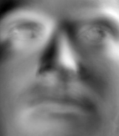
Eigenfaces: Faces as Points in High-D Space
2,410 face images, each $192 \times 168 = $ 32,256 pixels. Each face is a point in 32,256-dimensional space.
Goal: represent any face as a combination of a few basis faces (eigenfaces). PCA finds these basis directions.
Average Face
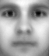
$\bar{\mathbf{x}} = \frac{1}{n}\sum \mathbf{x}^{(i)}$
First 8 Eigenfaces (Principal Components)
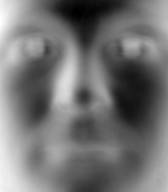
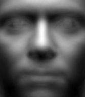
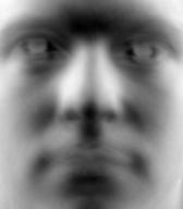
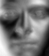
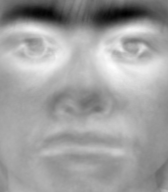
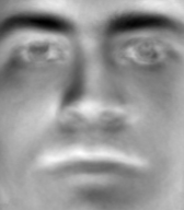
Each eigenface captures a different mode of variation (lighting, pose, expression).
Brunton & Kutz, Data-Driven Science and Engineering, Cambridge UP, 2019
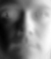
Face Reconstruction
Reconstruct a face using $k$ eigenfaces: $\hat{\mathbf{x}} = \bar{\mathbf{x}} + \sum_{i=1}^k c_i\,\mathbf{u}_i$
Original
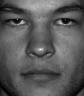
Reconstruction
Brunton & Kutz, Data-Driven Science and Engineering, Cambridge UP, 2019
Scree Plot: How Many Components?
The scree plot shows singular values (or eigenvalues) in decreasing order. Look for the "elbow".
• Cumulative variance ≥ 95%
• "Elbow" in scree plot
• Cross-validate for prediction
Summary
The key equation:
$\mathbf{X} = \mathbf{U}\boldsymbol{\Sigma}\mathbf{V}^\top$
No need to form $\mathbf{X}^\top\mathbf{X}$ explicitly.
Applications:
• Dimensionality reduction
• Image compression
• Denoising
• Feature extraction
• Visualization
What's Next?
What if the data is a time series?
What if we want to decompose dynamics, not just static data?
Next lecture: Linear Dynamical Systems & DMD