Linear Dynamical Systems
& Dynamic Mode Decomposition
From Eigenvalues to Data-Driven Dynamics

ML for Science and Engineering — Lecture 10

Schmid, "Dynamic mode decomposition of numerical and experimental data," J. Fluid Mech. 656, 2010
Brunton & Kutz, Data-Driven Science and Engineering, Cambridge UP, 2019

Coupled Oscillators

Two masses connected by springs: a classic linear system.

$m_1 \ddot{x}_1 = -k_1 x_1 + k_2(x_2 - x_1)$
$m_2 \ddot{x}_2 = -k_2(x_2 - x_1) - k_3 x_2$

$\frac{d\mathbf{x}}{dt} = A\,\mathbf{x}$

$m_1=m_2=1,\; k_1=k_2=k_3=1,\; x_1(0)=1,\; x_2(0)=0$

            The matrix $A$ encodes all the physics. Two frequencies emerge from the coupling.
        

When Is a System Linear?

Linear: $A$ is constant

$\dot{\mathbf{x}} = A\,\mathbf{x}$

Coupled oscillators, circuits,
small perturbations, heat equation

Nonlinear: $A$ depends on state

$\dot{\mathbf{x}} = f(\mathbf{x})$

Pendulum (large angle), Lorenz,
Navier-Stokes, population dynamics

Even nonlinear systems are locally linear (linearization around fixed points). DMD exploits this idea globally.

Eigendecomposition of $A$

Any square matrix can be decomposed as

$A = V \Lambda V^{-1}$

Written out for an $n \times n$ matrix:

$$A = \underbrace{\begin{bmatrix} | & | & & | \\ \mathbf{v}_1 & \mathbf{v}_2 & \cdots & \mathbf{v}_n \\ | & | & & | \end{bmatrix}}_{V} \underbrace{\begin{bmatrix} \lambda_1 & & \\ & \lambda_2 & \\ & & \ddots & \\ & & & \lambda_n \end{bmatrix}}_{\Lambda} \underbrace{\begin{bmatrix} \text{---} & \mathbf{w}_1^T & \text{---} \\ \text{---} & \mathbf{w}_2^T & \text{---} \\ & \vdots & \\ \text{---} & \mathbf{w}_n^T & \text{---} \end{bmatrix}}_{V^{-1}}$$

$\mathbf{v}_i$ = eigenvectors (columns of $V$)

Mode shapes: how components move together

$\lambda_i$ = eigenvalues (diagonal of $\Lambda$)

Growth rates: how fast each mode evolves

For symmetric $A$: eigenvectors are orthogonal and $V^{-1} = V^T$.

The Decoupling Trick

Starting from $\dot{\mathbf{x}} = A\mathbf{x}$, substitute $A = V\Lambda V^{-1}$:

$\dot{\mathbf{x}} = V \Lambda V^{-1}\, \mathbf{x}$

Multiply both sides on the left by $V^{-1}$:

$V^{-1}\dot{\mathbf{x}} = \Lambda\, V^{-1}\mathbf{x}$

Define a new variable $\mathbf{z} = V^{-1}\mathbf{x}$, so $\dot{\mathbf{z}} = V^{-1}\dot{\mathbf{x}}$:

$\dot{\mathbf{z}} = \Lambda\, \mathbf{z}$

Since $\Lambda$ is diagonal, each component decouples: $\dot{z}_i = \lambda_i\, z_i \;\;\Longrightarrow\;\; z_i(t) = z_i(0)\,e^{\lambda_i t}$

For symmetric $A$: $V^{-1} = V^T$, so the change of basis is just a rotation.

What Do Eigenvalues Tell Us?

For $z_i(t) = z_i(0)\,e^{\lambda_i t}$, the eigenvalue $\lambda_i$ controls the behavior:

$\lambda > 0$ (real)

Exponential growth

$\lambda < 0$ (real)

Exponential decay

$\lambda = \sigma \pm i\omega$

Oscillation (± growth/decay)

$e^{(\sigma + i\omega)t} = e^{\sigma t}\bigl(\cos\omega t + i\sin\omega t\bigr)$

Eigenvalue Plane

Click the complex plane to place an eigenvalue $\lambda$. See the resulting trajectory $z(t) = e^{\lambda t}$.

Click the plane or use a preset to explore eigenvalue behavior.

Example: Coupled Oscillators

For our spring-mass system with $m_1=m_2=1$, $k_1=k_2=k_3=1$:

The stiffness matrix $K$ has eigenvalues $\mu_i$ (stiffness per mode).

Natural frequencies: $\omega_i = \sqrt{\mu_i}$. System eigenvalues: $\lambda_i = \pm\, i\omega_i$.

Mode 1:   $\mu_1 = 1,\; \omega_1 = 1,\; \lambda = \pm i$

                    $\mathbf{v}_1 = \begin{bmatrix} 1 \\ 1 \end{bmatrix}$  
                    In-phase: both masses move together

Mode 2:   $\mu_2 = 3,\; \omega_2 = \sqrt{3},\; \lambda = \pm i\sqrt{3}$

                    $\mathbf{v}_2 = \begin{bmatrix} 1 \\ -1 \end{bmatrix}$  
                    Out-of-phase: masses move oppositely

All $\lambda_i$ are pure imaginary → oscillation with no growth or decay.

The full solution is a superposition:

$\mathbf{x}(t) = c_1 \cos(\omega_1 t)\,\mathbf{v}_1 + c_2 \cos(\omega_2 t)\,\mathbf{v}_2$

With $x_1(0) = 1, x_2(0) = 0$: $c_1 = c_2 = \tfrac{1}{2}$

Back to $\mathbf{x}$: Superposition of Modes

The general solution in original coordinates:

$\mathbf{x}(t) = \sum_{i=1}^n c_i\, e^{\lambda_i t}\, \mathbf{v}_i$

                Each mode $\mathbf{v}_i$ evolves independently at rate $\lambda_i$.

                The motion is their superposition.

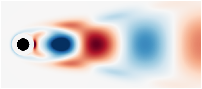
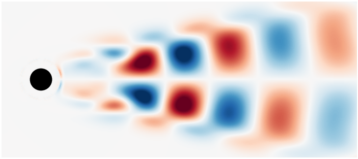
But what if we don't know $A$? What if we only have data?

Flow Past a Cylinder

Fluid flowing past a cylinder produces vortex shedding: alternating vortices behind the obstacle.

t = 0

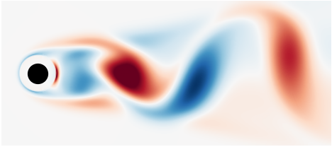
Mean-subtracted vorticity: oscillating vortex street

Data: 449 × 199 grid = 89,351 values per snapshot, 151 time steps.

            Each snapshot is a vector $\mathbf{x}_i \in \mathbb{R}^{89{,}351}$.

Brunton & Kutz, Data-Driven Science and Engineering, Cambridge UP, 2019

The Snapshot Matrix & Its SVD

Stack each snapshot as a column to form the data matrix $X$, then decompose it:

$X = \begin{bmatrix} | & | & & | \\ \mathbf{x}_1 & \mathbf{x}_2 & \cdots & \mathbf{x}_m \\ | & | & & | \end{bmatrix} \;\approx\; U_r\,\Sigma_r\, V_r^T$

Truncated SVD: keep only the $r$ largest singular values (rank-$r$ approximation of $X$).

$$X \;\approx\; \underbrace{\begin{bmatrix} | & | & & | \\ \mathbf{u}_1 & \mathbf{u}_2 & \cdots & \mathbf{u}_r \\ | & | & & | \end{bmatrix}}_{U_r \;\in\; \mathbb{R}^{n \times r}} \underbrace{\begin{bmatrix} \sigma_1 & & \\ & \sigma_2 & \\ & & \ddots \\ & & & \sigma_r \end{bmatrix}}_{\Sigma_r \;\in\; \mathbb{R}^{r \times r}} \underbrace{\begin{bmatrix} \text{---} & \mathbf{v}_1^T & \text{---} \\ \text{---} & \mathbf{v}_2^T & \text{---} \\ & \vdots & \\ \text{---} & \mathbf{v}_r^T & \text{---} \end{bmatrix}}_{V_r^T \;\in\; \mathbb{R}^{r \times m}}$$

$\mathbf{u}_i \in \mathbb{R}^{n}$: spatial modes

                    Orthogonal patterns in space, discovered from data. Each can be reshaped back to the spatial grid.

$\sigma_i$: singular values
Ranked by energy: $\sigma_1 \geq \sigma_2 \geq \cdots \geq 0$. Measure how important each mode is.

$\mathbf{v}_i^T \in \mathbb{R}^{m}$: temporal modes
How each spatial pattern evolves over time. Orthogonal time series.

            Like Fourier analysis discovers sine/cosine modes, SVD discovers the optimal orthogonal basis directly from the data.

            Both in space ($\mathbf{u}_i$) and time ($\mathbf{v}_i$).

SVD Modes of the Flow

Spatial modes (columns of $U$, reshaped to 449×199)

$\mathbf{u}_1$

$\mathbf{u}_2$

$\mathbf{u}_3$

$\mathbf{u}_4$

$\mathbf{u}_5$

$\mathbf{u}_6$

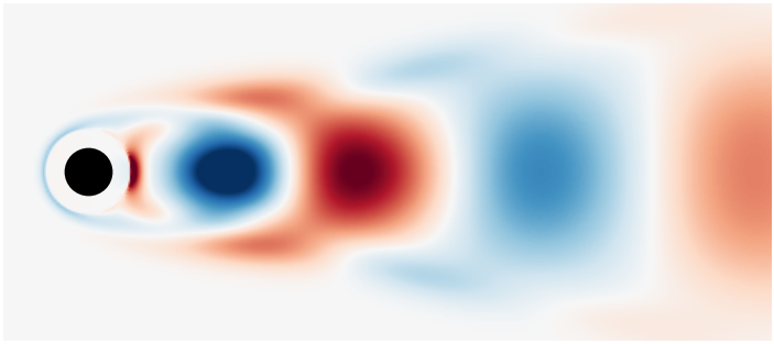
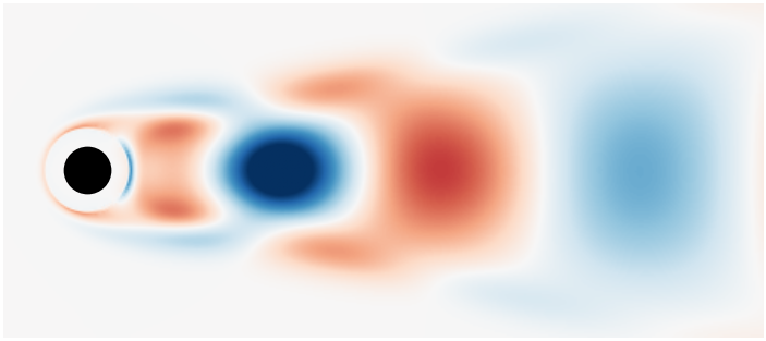
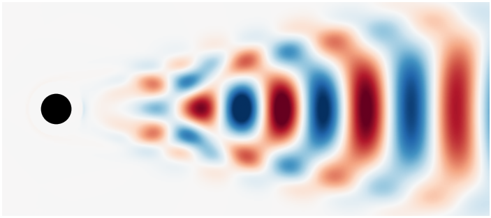
Each $\mathbf{u}_i \in \mathbb{R}^{89{,}351}$ is reshaped to 449×199 for display. Orthogonal, ranked by $\sigma_i$.

Temporal modes $\sigma_i \mathbf{v}_i^T$ (weighted rows of $V^T$)

                    The temporal modes look nearly sinusoidal for this periodic flow, but SVD does not enforce single-frequency behavior.
                    In general, each SVD mode can mix multiple frequencies
                    — SVD maximizes variance, not dynamical coherence.
                

Can we find modes where each captures a single, well-defined frequency?
→ Dynamic Mode Decomposition

From Time Series to a Dynamical Model

If the dynamics are (approximately) linear, then each snapshot maps to the next:

$\mathbf{x}_{i+1} = A\, \mathbf{x}_i$

Stack snapshots into two matrices:

$X = \begin{bmatrix} | & | & & | \\ \mathbf{x}_1 & \mathbf{x}_2 & \cdots & \mathbf{x}_{m-1} \\ | & | & & | \end{bmatrix}$

One-step-forward matrix:

$X' = \begin{bmatrix} | & | & & | \\ \mathbf{x}_2 & \mathbf{x}_3 & \cdots & \mathbf{x}_{m} \\ | & | & & | \end{bmatrix}$

The relationship $X' = AX$ holds column-by-column. Can we find $A$?

Solving for $A$

If $X' = AX$, how can we recover $A$?

We need some kind of "inverse" of $X$, but $X$ is rectangular ($n \times (m{-}1)$).

The pseudo-inverse $X^\dagger$ gives the least-squares solution:

$A = X'\, X^\dagger$

Using the SVD $X = U\Sigma V^T$, the pseudo-inverse is $X^\dagger = V\Sigma^{-1}U^T$, so:

$A = X'\, V\, \Sigma^{-1}\, U^T$

Problem: $A$ is $n \times n$ (e.g., $89{,}351 \times 89{,}351$ = 8 billion entries).
We cannot even store it, let alone eigendecompose it. We need a smarter approach.

The Low-Rank Projection

If the data lives in a low-dimensional subspace, we don't need the full $A$. Project onto the dominant $r$ SVD modes:

We want eigenvectors of $A$, but $A$ is $n \times n$. Instead, define a reduced operator:

$\tilde{A} = U_r^T\, A\, U_r$

$U_r$ projects from $\mathbb{R}^n$ into the $r$-dimensional subspace; $U_r^T$ projects back. $\tilde{A}$ is only $r \times r$.

Substituting $A = X' V \Sigma^{-1} U^T$ and truncating:

$\tilde{A} = U_r^T\, X'\, V_r\, \Sigma_r^{-1}$

For the cylinder flow: $\tilde{A}$ is $21 \times 21$ instead of $89{,}351 \times 89{,}351$. We can eigendecompose this.

SVD Spectrum: Low-Rank Structure

Does the cylinder flow data actually have low-rank structure? The SVD spectrum of $X$ confirms it:

The spectrum drops sharply. Most energy is in the first ~21 modes. The low-rank projection with $r = 21$ captures nearly all the dynamics.

DMD: Steps 1–2

Step 1: SVD of the data matrix

                $X = U\Sigma V^T$   →   truncate to rank $r$

This identifies the $r$-dimensional subspace where the dynamics live.

Step 2: Project the dynamics onto this subspace

                $\tilde{A} = U_r^T\, X'\, V_r\, \Sigma_r^{-1}$

$\tilde{A}$ is $r \times r$ — it captures how the system evolves within the dominant subspace.

Why does this work? If the data is truly low-rank, then $\tilde{A}$ is a faithful representation of $A$ restricted to the subspace that matters. Modes outside this subspace contribute negligible energy.

DMD: Steps 3–4

Step 3: Eigendecompose $\tilde{A}$

                $\tilde{A}\, W = W\, \Lambda$

$W$ = eigenvectors of $\tilde{A}$, $\Lambda = \text{diag}(\lambda_1, \ldots, \lambda_r)$. This is cheap: only $r \times r$.

Step 4: Recover full-space DMD modes

                $\Phi = X'\, V_r\, \Sigma_r^{-1}\, W$

Each column $\boldsymbol{\phi}_i$ is a spatial pattern in the original $n$-dimensional space.

Why $\Phi = X' V_r \Sigma_r^{-1} W$? The eigenvectors of $\tilde{A}$ live in the $r$-dimensional projected space. To lift them back to the full space, we use $X' V_r \Sigma_r^{-1}$, which maps from the reduced to the original coordinates. These are called exact DMD modes.

Dynamic Mode Decomposition in Python


def DMD(X, Xprime, r):
    # Step 1: SVD of X, truncate to rank r
    U, S, Vt = np.linalg.svd(X, full_matrices=False)
    Ur, Sr, Vtr = U[:, :r], np.diag(S[:r]), Vt[:r, :]

    # Step 2: Project dynamics onto SVD basis
    Atilde = Ur.T @ Xprime @ Vtr.T @ np.linalg.inv(Sr)

    # Step 3: Eigendecomposition of reduced operator
    Lambda, W = np.linalg.eig(Atilde)

    # Step 4: Recover full-space DMD modes
    Phi = Xprime @ Vtr.T @ np.linalg.inv(Sr) @ W

    return Phi, Lambda

            Four lines of linear algebra. The SVD from Lecture 9 does all the heavy lifting.
        

The DMD Reconstruction

DMD gives us modes $\boldsymbol{\phi}_i$, eigenvalues $\lambda_i$, and amplitudes $b_i$.

$\mathbf{x}(t) \;=\; \sum_{i=1}^{r}\, b_i\, \lambda_i^{\,t}\, \boldsymbol{\phi}_i$

$\boldsymbol{\phi}_i$ = spatial mode

A coherent spatial pattern (like an eigenface for dynamics).

$\lambda_i$ = eigenvalue

$|\lambda_i|$ controls growth/decay. $\angle\lambda_i$ is the oscillation frequency. We use $\lambda_i^t$ (not $e^{\lambda t}$) because this is discrete-time: snapshots at integer steps.

$b_i$ = amplitude

How much each mode contributes. Computed from the initial condition: $\mathbf{x}_1 = \Phi\,\mathbf{b}$, so $\mathbf{b} = \Phi^\dagger \mathbf{x}_1$.

Discrete vs continuous time:
Continuous: $e^{\lambda t}$ (imaginary axis = stability)
Discrete: $\lambda^t$ (unit circle = stability)
Connected by $\lambda_{\text{cont}} = \frac{\ln \lambda_{\text{disc}}}{\Delta t}$

DMD Eigenvalues

The 21 DMD eigenvalues in the complex plane. Points near the unit circle are persistent modes.

Discrete-time interpretation:

                    $|\lambda| < 1$: decaying

                    $|\lambda| = 1$: neutral

                    $|\lambda| > 1$: growing

                    $\angle\lambda$: oscillation frequency

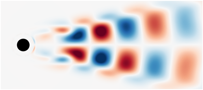
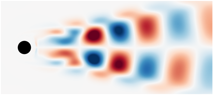
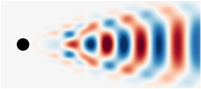
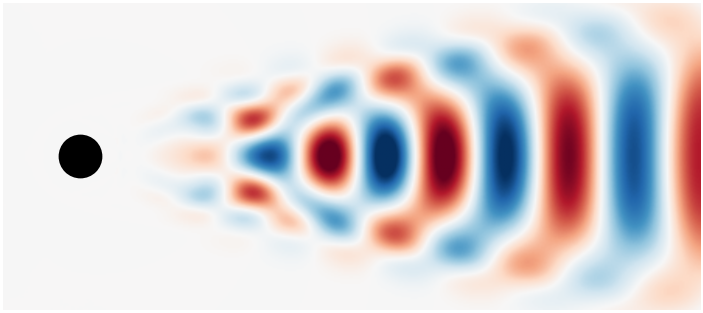
Notice the conjugate pairs: each pair $\lambda, \bar{\lambda}$ produces a real-valued oscillation.

Hover over a point to see its frequency and growth rate.

DMD Spatial Modes

The columns of $\Phi$: each mode captures a coherent spatial oscillation pattern.

Mode 1:

Mode 2:

Mode 3:

Mode 4:

Mode 5:

Mode 6:

            Each $\boldsymbol{\phi}_i$ shows Re($\boldsymbol{\phi}_i$). The spatial structure captures where vortices form.
            Modes come in conjugate pairs with the same spatial pattern but opposite phase.
        

DMD Temporal Dynamics

Each mode oscillates at its own frequency: $b_i\,\lambda_i^t$

Key property: Each DMD mode has a single, well-defined frequency.

                    The eigenvalue $\lambda_i$ determines that frequency exactly.

                    Compare with SVD temporal modes ($\sigma_i \mathbf{v}_i^T$),
                    which can mix multiple frequencies in each mode.
                

SVD vs DMD: Comparing Modes

How do the temporal modes from SVD and DMD compare?

SVD temporal modes ($\sigma_i \mathbf{v}_i^T$)

DMD temporal modes (Re($b_i \lambda_i^t$))

SVD modes are eigenvectors of $X^TX$ (covariance).

                    • Orthogonal

                    • Maximize captured variance

                    • Can mix multiple frequencies per mode

DMD modes are eigenvectors of $A$ (dynamics operator).
• Not necessarily orthogonal
• Each mode has a single frequency
• Dynamically coherent structures

DMD Reconstruction

How many modes do we need for a good reconstruction?

Original snapshot at $t=100$

DMD reconstruction at $t=100$

Rank: r = 21

With just 21 modes (out of 89,351 dimensions), DMD reconstructs the flow with <0.2% error.

Beyond Dynamic Mode Decomposition

Koopman Operator

For a nonlinear system $\dot{\mathbf{x}} = \mathbf{f}(\mathbf{x})$, let $F$ be the flow map that advances the state one step: $\mathbf{x}_{k+1} = F(\mathbf{x}_k)$.

For any scalar observable $g(\mathbf{x})$, the Koopman operator advances it:

$\mathcal{K}\, g(\mathbf{x}) = g\bigl(F(\mathbf{x})\bigr)$

$\mathcal{K}$ is linear (even though $F$ is not). Extended DMD approximates $\mathcal{K}$ by lifting the state with nonlinear features $\boldsymbol{\psi}(\mathbf{x})$.

	DMD	SINDy
Assumes	Linear dynamics	Sparse nonlinear
Method	Spectral decomp.	Sparse regression
Output	Global modes	Local equations
Scales to	Very high dim.	Low-moderate dim.

                    DMD finds the best linear model.
SINDy (Lecture 8) finds sparse nonlinear equations.
                

Summary

Linear Dynamical Systems: $\dot{\mathbf{x}} = A\mathbf{x}$

            Eigenvalues of $A$ control growth, decay, and oscillation. Each mode evolves independently.

Dynamic Mode Decomposition: Given snapshots, find $A$ efficiently via SVD projection.
4 steps: SVD → project → eigendecompose → recover modes.

Result: Spatial modes $\boldsymbol{\phi}_i$, eigenvalues $\lambda_i$, and amplitudes $b_i$.
From each $\lambda_i$: frequency $\omega_i = \angle\lambda_i$ and growth/decay from $|\lambda_i|$.
Data-driven decomposition: $\mathbf{x}(t) = \sum b_i \lambda_i^t \boldsymbol{\phi}_i$.

Ref: Schmid (2010), J. Fluid Mech. | Brunton & Kutz (2019) Ch. 7

Linear Dynamical Systems& Dynamic Mode Decomposition From Eigenvalues to Data-Driven Dynamics