Deep Learning for Time Series

From Ising Models to Recurrent Neural Networks

ML for Science and Engineering — Lecture 17
Joseph Bakarji

Where We Are

We have been building a toolkit for modeling dynamical systems from data:

What we have

ODE discretization: $x_{k+1} = f(x_k)$

SVD/POD for spatial modes

DMD for linear dynamics

SINDy for sparse equations

What if we don't know the structure?
What if the dynamics are too complex for a sparse model?
Can we learn $f$ directly from data using neural networks?

Key insight: Discretized ODEs are already recurrent: the next state depends on the current state. Neural networks can generalize this idea.

The Recurrence Idea

Every time-stepping scheme is an autoregressive model:

$$\text{Forward Euler:} \quad x_{k+1} = x_k + \Delta t \cdot f(x_k)$$

$$\text{General autoregressive:} \quad x_{k+1} = g(x_k, x_{k-1}, \ldots, x_{k-n})$$

Design question: What if $g$ includes learnable nonlinear transformations and operates in a hidden state space rather than the observable space?
        

This is the central idea behind recurrent neural networks. But the story starts much earlier, with physics.

Part I: Physics Roots

The Ising Model, Hopfield Networks, and Boltzmann Machines

How statistical mechanics inspired the first neural network architectures

The Ising Model (Lenz 1920, Ising 1925)

A model from statistical mechanics: a 2D grid of spins, each either "up" $(+1)$ or "down" $(-1)$. Neighboring spins want to align. The model was designed to explain ferromagnetism: how local interactions produce global order.

$$E = -J \sum_{\langle i,j \rangle} s_i s_j - h \sum_i s_i$$

$s_i \in \{-1, +1\}$ = spin at site $i$
$J > 0$ = coupling (scalar); favors aligned neighbors
$h$ = external magnetic field (scalar)
$\langle i,j \rangle$ = nearest-neighbor pairs only

The system evolves to minimize energy.
At high temperature $T$: thermal noise dominates, random spins
At low temperature: energy dominates, aligned spins
At $T_c \approx 2.27 J/k_B$: phase transition!

Temperature $T$ 2.27

Ising Model: The Algorithm

The Metropolis-Hastings algorithm simulates the Ising model at temperature $T$:

Algorithm (one sweep):

                    For each spin $s_i$ in random order:

                    1. Compute energy change if we flip it:

                    $\quad \Delta E = 2 J \, s_i \sum_{j \in \text{neighbors}} s_j$

                    2. If $\Delta E \leq 0$: flip (lower energy)

                    3. If $\Delta E > 0$: flip with probability $e^{-\Delta E / T}$

At equilibrium, the probability of a configuration follows the Boltzmann distribution: $P(\{s\}) = \frac{1}{Z} e^{-E(\{s\})/T}$

import numpy as np

def ising_step(grid, T, J=1.0):
    N = grid.shape[0]
    for _ in range(N * N):
        i, j = np.random.randint(N, size=2)
        s = grid[i, j]
        # Sum of 4 nearest neighbors
        neighbors = (grid[(i-1)%N, j] +
                     grid[(i+1)%N, j] +
                     grid[i, (j-1)%N] +
                     grid[i, (j+1)%N])
        dE = 2 * J * s * neighbors
        if dE <= 0 or np.random.rand() < np.exp(-dE / T):
            grid[i, j] = -s
    return grid

Full notebook with exercises available after this section

The Ising Model

↓ .ipynb Open in Colab

The Ising Model: From Statistical Physics to Neural Networks

The Ising model is the simplest model of a magnetic material. It was proposed by Wilhelm Lenz in 1920 and solved analytically in 1D by his student Ernst Ising in 1925. Despite its simplicity, it exhibits phase transitions and connects directly to Hopfield networks and Boltzmann machines.

The Model

A lattice of spins $s_i \in {-1, +1}$ with nearest-neighbor coupling:

$$E({s}) = -J \sum_{\langle i,j \rangle} s_i s_j$$

where $J > 0$ favors alignment (ferromagnetic). At temperature $T$, configurations follow the Boltzmann distribution:

$$P({s}) = \frac{1}{Z} e^{-E({s})/T}$$

▼Python

import numpy as np
import matplotlib.pyplot as plt
from matplotlib import animation
from IPython.display import HTML
# Grid size
N = 50
def init_grid(N, p=0.5):
 """Random initial spin configuration."""
return np.where(np.random.rand(N, N) < p, 1, -1)
def ising_step(grid, T, J=1.0):
 """One Monte Carlo sweep: N^2 random single-spin updates."""
N = grid.shape[0]
for _ in range(N * N):
i, j = np.random.randint(N, size=2)
s = grid[i, j]
# Sum of 4 nearest neighbors (periodic boundaries)
neighbors = (grid[(i-1)%N, j] + grid[(i+1)%N, j] +
grid[i, (j-1)%N] + grid[i, (j+1)%N])
dE = 2 * J * s * neighbors
# Metropolis criterion
if dE <= 0 or np.random.rand() < np.exp(-dE / T):
grid[i, j] = -s
return grid

Phase Transition

The 2D Ising model has a critical temperature $T_c \approx 2.27$ (in units of $J/k_B$).

$T < T_c$: Ordered phase — most spins align (spontaneous magnetization)
$T > T_c$: Disordered phase — spins point randomly (paramagnetic)
$T = T_c$: Critical point — fluctuations at all scales, power-law correlations

Let's simulate the Ising model at three temperatures and watch the dynamics.

▼Python

# Simulate at three temperatures
temperatures = [1.5, 2.27, 4.0]
labels = [f'T = {T} ({name})' for T, name in
zip(temperatures, ['ordered', 'critical', 'disordered'])]
n_steps = 100
fig, axes = plt.subplots(1, 3, figsize=(14, 4.5))
for ax, T, label in zip(axes, temperatures, labels):
grid = init_grid(N)
# Equilibrate
for _ in range(n_steps):
grid = ising_step(grid, T)
ax.imshow(grid, cmap='coolwarm', vmin=-1, vmax=1, interpolation='nearest')
ax.set_title(label, fontsize=12)
ax.axis('off')
plt.suptitle('Ising Model After 100 Monte Carlo Sweeps', fontsize=14)
plt.tight_layout()
plt.show()

Measuring the Magnetization

The order parameter is the average magnetization:

$$m = \frac{1}{N^2} \left| \sum_i s_i \right|$$

Near $T_c$, it drops from $m \approx 1$ to $m \approx 0$. Let's trace $m(T)$.

▼Python

# Sweep temperature and measure magnetization
T_range = np.linspace(1.0, 4.0, 25)
mag_avg = []
n_equil = 50 # equilibration sweeps
n_sample = 30 # measurement sweeps
for T in T_range:
grid = init_grid(N)
# Equilibrate
for _ in range(n_equil):
grid = ising_step(grid, T)
# Measure
mags = []
for _ in range(n_sample):
grid = ising_step(grid, T)
mags.append(np.abs(grid.mean()))
mag_avg.append(np.mean(mags))
plt.figure(figsize=(8, 4))
plt.plot(T_range, mag_avg, 'o-', color='#61afef', markersize=5)
plt.axvline(2.27, color='#e06c75', linestyle='--', label=r'$T_c \approx 2.27$')
plt.xlabel('Temperature $T$', fontsize=12)
plt.ylabel(r'Magnetization $\langle |m| \rangle$', fontsize=12)
plt.title('Phase Transition in the 2D Ising Model', fontsize=13)
plt.legend(fontsize=11)
plt.grid(alpha=0.3)
plt.show()

Connection to Neural Networks

The Ising model is the direct ancestor of:

Physics	Neural Networks
Spin $s_i \in {-1, +1}$	Neuron activation
Coupling $J_{ij}$	Synaptic weight $w_{ij}$
Energy $E({s})$	Loss / cost function
Boltzmann dist. $e^{-E/T}$	Softmax / Gibbs sampling
Energy minimization	Learning

Hopfield (1982): Replace the lattice with a fully connected graph. Local energy minima become stored memories.

Boltzmann machines (1985): Add hidden units. Train by adjusting $J_{ij}$ to match data statistics.

The mathematical framework is identical — only the interpretation changes.

Exercises

Critical slowing down: Measure how many sweeps it takes to reach equilibrium at $T = T_c$ vs. $T = 1.5$. Why is it slower near the critical point?
Energy vs. temperature: Plot the average energy $\langle E \rangle$ as a function of $T$. Compute the specific heat $C = \partial \langle E \rangle / \partial T$ and find its peak near $T_c$.
External field: Add an external magnetic field $h$ to the energy: $E = -J \sum s_i s_j - h \sum s_i$. How does the magnetization curve change?
Hopfield network: Modify the code so that $J_{ij}$ stores patterns via the Hebbian rule $J_{ij} = \frac{1}{P}\sum_{\mu=1}^P \xi_i^\mu \xi_j^\mu$. Initialize the grid near a stored pattern and watch it converge.

Scroll to explore · code cells are collapsible

From Spins to Neurons: Hopfield Networks (1982)

John Hopfield's insight: replace the Ising lattice with a fully connected network. Instead of nearest-neighbor coupling, every neuron connects to every other. The energy landscape has local minima that serve as stored memories.

$$E = -\frac{1}{2} \sum_{i \neq j} W_{ij} s_i s_j - \sum_i b_i s_i$$

Same energy as Ising, but with all-to-all learned weights $W_{ij}$ instead of uniform nearest-neighbor coupling $J$.

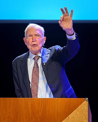
2024 Nobel Prize in Physics awarded to John Hopfield and Geoffrey Hinton "for foundational discoveries and inventions that enable machine learning with artificial neural networks."

John Hopfield

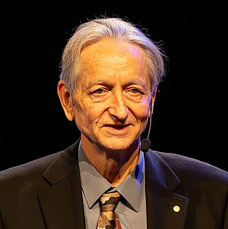
Geoffrey Hinton

Nobel Prize in Physics 2024

Photos: Wikimedia Commons (CC BY 4.0)

How Hopfield Networks Work

The network operates as an associative memory: given a corrupted input, it recovers the closest stored pattern.

Setup:

$s_i \in \{-1, +1\}$: neuron states (like pixel values in an image)

$W_{ij}$: connection weights (computed from training data)

Patterns $\xi^\mu$: binary images we want to store

Step 1 — Store: Compute weights from $M$ patterns:
$W_{ij} = \frac{1}{N} \sum_{\mu=1}^{M} \xi_i^\mu \xi_j^\mu$
(This is like an autocorrelation: neurons that co-activate get stronger connections)

Step 2 — Recall: Initialize $s$ with a corrupted pattern. Update each neuron:

                    $s_i \leftarrow \text{sign}\!\left(\sum_j W_{ij} s_j\right)$

                    Each update decreases energy $\Rightarrow$ converges to nearest minimum = nearest stored pattern

Click "Store" to begin

Hopfield: Capacity and Limitations

Capacity limit (McEliece et al. 1987):
At most $\sim 0.138 N$ patterns for $N$ neurons.
Beyond this: spin-glass phase with spurious attractors (false memories).

Limitations of classical Hopfield:

Low capacity: only $O(N)$ patterns
Binary states only ($\pm 1$)
Spurious attractors (mixture states, reversed patterns)
No hidden representation

Why study Hopfield networks?
1. First architecture where physics principles (energy minimization) directly defined computation
2. The design logic generalizes: define an energy, let the system minimize it
3. Direct mathematical ancestor of transformers (next slide)

Research Connection: Modern Hopfield $\rightarrow$ Transformers

Ramsauer et al. (2021) showed that with continuous states and a log-sum-exp energy, the Hopfield update rule becomes:

$$\xi^{\text{new}} = X \cdot \text{softmax}(\beta \, X^T \xi)$$

Modern Hopfield

                Query state $\xi$, stored patterns $X$

                Inverse temperature $\beta$

                Storage: $\exp(O(d))$ patterns

Transformer Attention
Query $Q$, Keys $K$, Values $V$
$\beta = 1/\sqrt{d_k}$
$\text{softmax}(QK^T\!/\sqrt{d_k}) \cdot V$

The punchline: Each attention head in a transformer performs one step of modern Hopfield network retrieval. The lineage Ising $\rightarrow$ Hopfield $\rightarrow$ Transformers is mathematically precise. (We may revisit transformers in a later lecture.)

Boltzmann Machines: Adding Stochasticity (Optional)

Geoffrey Hinton and Terrence Sejnowski (1985) extended Hopfield networks with two ingredients:

1. Stochastic updates (finite temperature)

                    Instead of deterministic $s_i = \text{sign}(h_i)$, flip with probability:

                    $$P(s_i = 1) = \sigma\!\left(\frac{h_i}{T}\right) = \frac{1}{1 + e^{-h_i/T}}$$
                    This lets the network escape local minima (like simulated annealing).

2. Hidden units
Split neurons into:
Visible $v$ = observed data (e.g., time series windows, sensor readings, image pixels)
Hidden $h$ = latent features the model discovers (temporal patterns, modes)

Boltzmann Machines: The Math

A Restricted Boltzmann Machine (RBM) has no connections within the same layer (bipartite graph):

$$E(v, h) = -\underbrace{a^T v}_{\text{visible bias}} - \underbrace{b^T h}_{\text{hidden bias}} - \underbrace{v^T W h}_{\text{interaction}}$$

The probability of a data configuration follows the Boltzmann distribution: $$P(v, h) = \frac{1}{Z} e^{-E(v,h)}, \qquad Z = \sum_{v,h} e^{-E(v,h)}$$

Concrete examples:

Images: $v$ = 784 pixels (MNIST). RBM learns digit-like patterns.

Time series: $v$ = a window of $T$ observations $[x_t, \ldots, x_{t+T}]$. RBM learns temporal motifs and transition probabilities.

Why "restricted"? No connections within visible or hidden layers means units are conditionally independent:
$P(h_j = 1 | v) = \sigma(b_j + \sum_i W_{ij} v_i)$
This makes sampling efficient (block Gibbs).

Training Boltzmann Machines

Goal: maximize the probability the model assigns to real data. The gradient has a beautiful structure:

$$\frac{\partial \log P(v)}{\partial W_{ij}} = \underbrace{\langle v_i h_j \rangle_{\text{data}}}_{\text{positive phase: what the data looks like}} - \underbrace{\langle v_i h_j \rangle_{\text{model}}}_{\text{negative phase: what the model thinks data looks like}}$$

Positive phase (easy)
Clamp $v$ to real data. Sample $h$ from $P(h|v)$.
Measures correlations in real data.

Negative phase (hard!)
Sample from full model $P(v,h)$. Requires MCMC to equilibrium.
Contrastive Divergence (Hinton 2002): just 1 Gibbs step!

Free energy: $F(v) = -a^T v - \sum_j \log(1 + e^{b_j + \sum_i v_i W_{ij}})$. Note the $\log(1 + e^x)$ = softplus, the smooth ancestor of ReLU!
        

Deep Belief Networks (Hinton et al. 2006) stacked RBMs layer-by-layer, kickstarting the deep learning revolution. Superseded by dropout, batch norm, and ReLU by ~2012.

The Intellectual Lineage

Physics-inspired designs gave birth to modern deep learning:

Hopfield (1982)

Energy minimization
Associative memory

$\downarrow$

Modern Hopfield
$\rightarrow$ Transformers

Boltzmann (1985)

Gibbs distribution
Generative model

$\downarrow$

Pretraining
$\rightarrow$ VAEs, GANs, Diffusion

Ising (1920)

Phase transitions
Statistical mechanics

$\downarrow$

Energy-based learning
$\rightarrow$ Unifying framework

Design lesson: These architectures were derived from physical principles: energy minimization, statistical equilibrium, symmetry. Understanding the physics helps you understand why an architecture works, and how to invent new ones.
        

Part II: Recurrent Neural Networks

Learning dynamics in a hidden state space

The RNN Architecture

Introduce a hidden state $h_t$ that captures information beyond the current observation:

Hidden update:

$$h_t = \tanh(W_{hh} \, h_{t-1} + W_{xh} \, x_t + b_h)$$

Output / prediction:

$$\hat{x}_{t+1} = W_{hy} \, h_t + b_y$$

Loss: $\mathcal{L} = \sum_t \|\hat{x}_{t+1} - x_{t+1}\|^2$ — minimize prediction error across the sequence.

RNN in Action: Step by Step

Click Next to advance through the sequence. At each step, the hidden state $h_t$ absorbs the new input and produces a prediction.

Step 0 / 6

Further reading: Dobilas, S. (2022). "RNN: How to Successfully Model Sequential Data in Python." Towards Data Science. Link

RNN as a State-Space Model

The RNN is a nonlinear generalization of the discrete-time state-space model:

	Linear State-Space	RNN
State update	$h_{t+1} = A h_t + B x_t$	$h_t = \tanh(W_{hh} h_{t-1} + W_{xh} x_t)$
Output	$y_t = C h_t$	$\hat{x}_{t+1} = W_{hy} h_t$
Dynamics	$A$ (fixed matrix)	$W_{hh}$ (learned, nonlinear)
Input coupling	$B$ (fixed)	$W_{xh}$ (learned)
Readout	$C$ (fixed)	$W_{hy}$ (learned)

Key idea: The hidden state $h_t$ is a compressed representation of the entire input history. This is also the idea behind Hidden Markov Models (HMMs), where the latent state evolves stochastically and observations are noisy projections. RNNs make this deterministic and end-to-end differentiable.

Backpropagation Through Time (BPTT)

To train the RNN, we unroll through time and apply the chain rule. The gradient at time $t$ involves all earlier hidden states:

$$\frac{\partial \mathcal{L}_4}{\partial W_{hh}} = \frac{\partial \mathcal{L}_4}{\partial h_4} \cdot \frac{\partial h_4}{\partial W_{hh}}$$

$$\quad + \frac{\partial \mathcal{L}_4}{\partial h_4} \cdot \frac{\partial h_4}{\partial h_3} \cdot \frac{\partial h_3}{\partial W_{hh}}$$

$$\quad + \frac{\partial \mathcal{L}_4}{\partial h_4} \cdot \frac{\partial h_4}{\partial h_3} \cdot \frac{\partial h_3}{\partial h_2} \cdot \frac{\partial h_2}{\partial W_{hh}} \;+\; \cdots$$

Each step-to-step Jacobian: $\;\frac{\partial h_{k+1}}{\partial h_k} = W_{hh}^T \cdot \text{diag}(\tanh'(z_k))$, so:

$$\prod_{k=2}^{t} \frac{\partial h_{k}}{\partial h_{k-1}} = \prod_{k=2}^{t} W_{hh}^T \cdot \text{diag}(\tanh'(z_k))$$

Vanishing/exploding gradient: If $\|W_{hh}\| < 1$: product shrinks exponentially → early gradients vanish. If $\|W_{hh}\| > 1$: grows exponentially → gradients explode. Long-range dependencies become invisible to learning.

Vanishing Gradients: Interactive

The spectral radius $\rho(W_{hh})$ is the largest eigenvalue magnitude of $W_{hh}$. It controls how gradients scale through time: $\;\left|\frac{\partial h_k}{\partial h_0}\right| \sim \big(\rho(W_{hh}) \cdot \overline{\tanh'}\big)^k$

Spectral radius ρ(W_hh) 0.90

Sequence length T 20

Green zone: gradient large enough to update weights. Red zone: gradient below $10^{-2}$ — effectively zero. Effective rate = $\rho \times \overline{\tanh'} \approx \rho \times 0.65$.

LSTM: Solving the Vanishing Gradient

Hochreiter & Schmidhuber (1997) introduced gating mechanisms and a cell state highway:

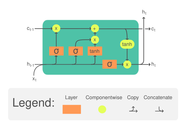
Source: Wikipedia (CC BY-SA 4.0)

Forget: $f_t = \sigma(W_f [h_{t-1}, x_t] + b_f)$

Input: $i_t = \sigma(W_i [h_{t-1}, x_t] + b_i)$

Candidate: $\tilde{c}_t = \tanh(W_c [h_{t-1}, x_t] + b_c)$

Cell update: $c_t = f_t \odot c_{t-1} + i_t \odot \tilde{c}_t$

Output: $o_t = \sigma(W_o [h_{t-1}, x_t] + b_o)$

Hidden: $h_t = o_t \odot \tanh(c_t)$

Why it works: $c_t = f_t \odot c_{t-1} + \ldots$ is additive. Gradients flow through $\prod_k f_k$ (forget gates near 1). No repeated $W_{hh}$ multiplication on the cell state highway.

Same idea as ResNet (He et al. 2015): $h_{l+1} = h_l + f(h_l)$. The skip connection lets gradients flow unimpeded. LSTM's cell highway (1997) predates ResNet by 18 years!
                

Part III: Reservoir Computing

What if you never train the recurrent weights?

Echo State Networks (Jaeger, 2001)

A radically different approach: the recurrent dynamics are random and fixed. Only a linear readout is trained.

Jaeger, H. (2001). "The echo state approach to analysing and training recurrent neural networks." GMD Report 148, German National Research Center for Information Technology.

Reservoir (fixed, random):
$h_{t+1} = \tanh(W_{\text{in}} x_{t+1} + W h_t)$

Output (trained, linear):
$y_t = W_{\text{out}} h_t$

$W_{\text{in}}$ (input $\rightarrow$ reservoir): random, fixed
$W$ (reservoir $\rightarrow$ reservoir): random, fixed
$W_{\text{out}}$ (reservoir $\rightarrow$ output): trained via ridge regression

Training: $W_{\text{out}} = Y H^T (H H^T + \beta I)^{-1}$
One linear solve. No backpropagation. Seconds, not hours.

The Echo State Property

For the reservoir to be useful, it must forget initial conditions:

Echo State Property:

                    $\|h(t) - h'(t)\| \to 0$ as $t \to \infty$

                    for any two initial states driven by the same input.

Sufficient condition: spectral radius $\rho(W) < 1$

                    (because $\tanh$ is Lipschitz-1, so $\|h_t - h'_t\| \leq \|W\| \cdot \|h_{t-1} - h'_{t-1}\|$)

Edge of chaos ($\rho \approx 1$):
Best performance at the boundary between order and chaos.

$\rho \ll 1$: short memory, strong nonlinearity
$\rho \to 1$: long memory, more linear
$\rho > 1$: risk of instability

Reservoir Dynamics: Interactive

A sinusoidal input $x(t)$ drives 4 reservoir neurons. Each neuron transforms the input differently via random weights. The spectral radius $\rho(W)$ controls how much memory the reservoir has.

Spectral radius ρ(W) 0.90

Input frequency 0.05

(draws new random $W$, $W_{\text{in}}$)

Low $\rho$: neurons quickly forget past input (short memory). High $\rho$ ($\approx 1$): richer nonlinear responses, longer memory. $\rho > 1$: unstable.

Physical Reservoir Computing

Any physical system with sufficient complexity, nonlinearity, and fading memory can be a reservoir:

Physical System	Reservoir Mechanism	Reference
Photonic circuits	Mach-Zehnder modulator + delay feedback	Larger et al. 2012
Mechanical networks	Mass-spring nonlinear coupling	Dion et al. 2018
Quantum systems	Interacting qubits, exponential Hilbert space	Fujii & Nakajima 2017
Biological neurons	Cortical microcircuits (Liquid State Machines)	Maass et al. 2002

Key insight: A single nonlinear node with delay feedback creates a virtual reservoir via time-multiplexing. Connects to delay-differential equations and Takens' embedding theorem.

Case Study: Predicting Chaos

Pathak et al., Physical Review Letters (2018)

The Kuramoto-Sivashinsky Equation

Developed independently by Kuramoto (1978, chemical oscillations) and Sivashinsky (1977, flame-front instabilities). It is one of the simplest PDEs exhibiting spatiotemporal chaos:

$$\frac{\partial u}{\partial t} = -u \frac{\partial u}{\partial x} - \frac{\partial^2 u}{\partial x^2} - \frac{\partial^4 u}{\partial x^4}$$

$-u \, u_x$: nonlinear advection — transfers energy between spatial scales

$-u_{xx}$: anti-diffusion — injects energy at small scales (destabilizing!)

$-u_{xxxx}$: hyper-diffusion — dissipates energy at the smallest scales

                    The balance produces chaos with positive Lyapunov exponents. The largest Lyapunov exponent $\lambda_{\max}$ measures the fastest rate of exponential divergence between nearby trajectories. The Lyapunov time $\tau_\lambda = 1/\lambda_{\max}$ is the timescale over which they diverge by a factor of $e$. Beyond a few $\tau_\lambda$, prediction is fundamentally impossible. How many Lyapunov times can we predict?

Simulated KS-like spatiotemporal pattern

Pathak et al.: Architecture & Results

Architecture (ESN applied to KS):

Input: $u(x, t)$ discretized to 64 spatial points

Reservoir: $h_{t+1} = \tanh(W_{\text{in}} \, u_t + W \, h_t)$, $N{=}5000$, $\rho{=}0.9$

Readout: $\hat{u}_{t+1} = W_{\text{out}} \, h_t$ trained by ridge regression

Prediction: feed $\hat{u}_{t+1}$ back as input (autonomous mode)

Results:
$\sim 8$ Lyapunov times of valid prediction
Correct Lyapunov exponent spectrum
Accurate long-term climate (statistics)

All with ridge regression. No backpropagation.

Pathak, J., Hunt, B., Girvan, M., Lu, Z., & Ott, E. (2018). "Model-free prediction of large spatiotemporally chaotic systems from data: A reservoir computing approach." Physical Review Letters, 120(2), 024102. doi:10.1103/PhysRevLett.120.024102

Architecture Comparison

Feature	Vanilla RNN	LSTM	ESN
Recurrent weights	Trained (BPTT)	Trained (BPTT)	Fixed random
Training cost	$O(N^2 T \cdot \text{epochs})$	$O(N^2 T \cdot \text{epochs})$	$O(N^2 T + N^3)$
Gradient issues	Vanishing / exploding	Mitigated (cell highway)	None (no BPTT)
Memory	Short	Long (gated)	$\leq N$ (hard limit)
Interpretability	Low	Low	High (linear readout)
Adaptability	Learned features	Learned features	Random features

Beyond: Modern Extensions

Neural ODEs

                    ResNet: $h_{k+1} = h_k + f(h_k)$

                    As layers $\to \infty$: $\frac{dh}{dt} = f(h, t)$

                    Chen et al. 2018

State Space Models
Mamba: structured SSM
$h' = Ah + Bx$, $y = Ch$
Linear recurrence, $O(N \log N)$

Transformers
Attention over full sequence
No explicit recurrence
Dominant in NLP

Next-Gen RC
Gauthier et al. 2021
No reservoir: polynomial features
of time-delay embeddings

GRU
Cho et al. 2014
Simplified LSTM: 2 gates
Often comparable performance

Temporal Fusion
Lim et al. 2021
Attention + LSTM hybrid
Multi-horizon forecasting

Summary: Design Principles

Era	Architecture	Core Idea	Physics Connection
1980s	Hopfield / Boltzmann	Energy minimization as computation	Ising model, stat mech
1990s	RNN / LSTM	Learned dynamics in hidden space	Dynamical systems, state-space
2000s	Echo State Networks	Random dynamics + linear readout	Edge of chaos, physical reservoirs
2020s	Transformers / SSMs	Attention = Hopfield retrieval	Modern Hopfield energy

The takeaway: Understanding these architectures is about understanding the design logic: what problem does each design choice solve? What tradeoff does it make? This is how you invent the next one.

References

Hopfield & Boltzmann

Hopfield (1982). Neural networks and physical systems with emergent collective computational abilities. PNAS.

Ramsauer et al. (2021). Hopfield networks is all you need. ICLR.

McEliece et al. (1987). The capacity of the Hopfield associative memory. IEEE TIT.

Hinton & Sejnowski (1983). Boltzmann machines. CVPR.

Hinton (2002). Contrastive divergence. Neural Computation.

Hinton et al. (2006). Deep belief nets. Neural Computation.

RNNs & LSTMs

Hochreiter & Schmidhuber (1997). Long short-term memory. Neural Computation.

Cho et al. (2014). GRU encoder-decoder. EMNLP.

Reservoir Computing

Jaeger (2001). Echo state networks. GMD Report 148.

Maass et al. (2002). Liquid state machines. Neural Computation.

Pathak et al. (2018). Predicting spatiotemporal chaos. PRL.

Dambre et al. (2012). Information processing capacity. Scientific Reports.

Gauthier et al. (2021). Next generation RC. Nature Comm.

Modern

Chen et al. (2018). Neural ODEs. NeurIPS.

LeCun et al. (2006). Energy-based learning. MIT Press.