Generalization and Feature Engineering
Introduction to Machine Learning
Six questions about data you have not seen
The houses from the linear regression lecture come back in Parts 4 and 5: first the same twenty, asked to predict the 2,905 they never saw, then random samples of the whole file.
Summary: the recipe so far
Everything after this lecture changes one line of that recipe: which \( h \) you are allowed to assume.
Given a new input, what’s the output?
| Input (size) | Output (price) |
|---|---|
| \( x^{(1)} \) | \( y^{(1)} \) |
| \( x^{(2)} \) | \( y^{(2)} \) |
| \( x^{(3)} \) | \( y^{(3)} \) |
| \( x^{(4)} \) | \( y^{(4)} \) |
| \( \vdots \) | \( \vdots \) |
Query \( x_q \) goes in, prediction \( y_p \) comes out.
Given new input, what’s the output?
Given the data, find a function \( h \), a.k.a. a hypothesis, that predicts outputs given inputs. \( h : \mathbb{R} \to \mathbb{R} \)
Given new input, what’s the output?
Given the data, find a function \( h \), a.k.a. a hypothesis, that predicts outputs given inputs. \( h : \mathbb{R} \to \mathbb{R} \)
How do you choose the hypothesis?
Given the data, find a function \( h \), a.k.a. a hypothesis, that predicts outputs given inputs. \( h : \mathbb{R} \to \mathbb{R} \)
Part 2 of 6
Two stories about fits
Can a fit be real with a low score, and wrong with a high one?
A Feature Built in 1885
Francis Galton measured 928 grown children and their parents, and had to invent a feature before he could plot anything.
Two parents, two numbers, one axis. The 1.08 scales mothers up before averaging, so that a tall mother and a tall father count the same. It is a modelling decision, made before any fitting, and it is baked into every number that follows.
Five families from the original table. 934 rows, 205 families.
Count the Points
There are 928 children in this plot. Nothing about the plot says so.
Galton rounded every height, so 928 measurements land on 102 positions. One position holds 48 children. Three quarters of the data sits under a dot that hides at least nine others.
Where the Word Comes From
The fitted line is flatter than the dashed line where a child simply matches the parent. That gap is the whole story.
Galton called this regression towards mediocrity. The field is named after this slope, in this dataset, being less than one.
Tall parents do have tall children. Just less tall. Short parents likewise, in the other direction.
A Fifth of the Variance, and a Whole Discipline
Correlation \( r = 0.459 \). Its square is the share of the variance in the child's height that the fit accounts for: residual over total, subtracted from one.
Spread of child heights, before and after the parents are taken into account.
A Model With a Date On It
von Foerster, Mora and Amiot, Science, 1960. Title: "Doomsday: Friday, 13 November, A.D. 2026".
They fitted world population with one curve:
Fitted on two thousand years of data, they got \( t_0 = 2026.87 \) and \( k = 0.99 \). The curve goes to infinity at \( t_0 \), and that date is a Friday.
To be fair to them: the paper was partly tongue in cheek. They were not predicting infinite people. They were arguing that the growth pattern of the previous two millennia was about to break. It did.
World population, 1700 to 2023. Our World in Data, vendored CSV.
Fit It Yourself, Then Look Forward
Set \( k = 1 \) and the model is a straight line in \( 1/N \), so this is one least squares fit.
Drag the cutoff and doomsday wanders from 2063 to 2039. It never admits it is wrong: \( R^2 \) stays above 0.99 throughout, highest at 2020, while the 2023 forecast drifts from 8.4 billion past 14.
What a Curve Cannot Know
Annual growth rate of world population.
Growth peaked at 2.2 per cent a year in the early 1960s and has fallen ever since: 1.36 in 2000, 0.88 in 2023. Births per woman fell as child mortality fell, incomes rose and cities grew.
Galton: \( R^2 = 0.21 \), and the finding is real.
von Foerster: \( R^2 = 0.99 \), and the model is wrong.
Read the original: Doomsday, Science 132 (1960). A modern critique: arXiv 0910.3056, and the end of hyperbolic growth.
Part 3 of 6
Features
How does a linear model draw a curve?
Assume a linear hypothesis
Assume a linear hypothesis
Example: construct a polynomial model
A curve, from a model that is linear in its parameters
Assume a linear hypothesis
Written out, the feature map is just a list of functions of \( x \), and the model is a weighted sum of them.
- Each \( \phi_j \) is a choice. Powers of \( x \) give a polynomial. Sines give a Fourier series. Indicator functions give a step model.
- The shapes. \( \phi(x) \in \mathbb{R}^{p}, \quad \theta \in \mathbb{R}^{p}, \quad h_\theta(x) \in \mathbb{R} \)
- Fitting is unchanged. Least squares on \( \phi(x) \) instead of on \( x \). Every formula you already have still applies.
Example: construct a polynomial model
Pick two features and nothing else:
\( \phi(x) = [x,\, x^3] \), the feature map
No constant term and no \( x^2 \): those are modelling choices, and they are choices you make before any fitting happens.
Part 4 of 6
Generalization
How do you know a model will work on data it has not seen?
How to choose \( \phi(x) \)? How to optimize over \( \phi(x) \)
Same data, same fitting procedure. The only thing that changed is which features you allowed.
The twenty houses, one degree at a time
The orange houses are the twenty from the linear regression lecture. The faint blue ones are the rest of Ames: data the fit never sees.
Each added power helps a little on the twenty and hurts everywhere else. Ten parameters still cannot pass through twenty scattered houses, so the curve spends its freedom where there are no houses, and past degree 4 its error on real houses runs into millions of dollars. The training error never warned you.
How can we tell if \( \phi(\cdot) \) is good?
The purpose of machine learning is to generalize to unseen data
The green points are the same points in all three panels. They were never used to fit anything.
How can we tell if \( \phi(\cdot) \) is good?
Define objective functions for each subset
Create a test set to evaluate the model
Split data:
Variance Bias Trade-off
Error as a function of complexity
- Training error falls as you add features, and keeps falling. It is not evidence of anything.
- Test error turns around. Everything to the left of the turn is bias, everything to the right is variance.
- You cannot see the turn from the training set alone. That is what the held-out data is for.
Both curves are measured, not drawn: each point is a least squares fit at that degree on the same data.
Other Hyperparameters
\( \phi \) is not the only unknown parameter over which we want to optimize
- \( T \): number of epochs, how long you train for.
- \( \eta \): step size, how far each update moves.
- \( \phi \): the feature vector, which functions of \( x \) the model is allowed to use.
A hyperparameter is a setting you choose before fitting, which the fit does not choose for you: the degree, the step size, the number of epochs (passes through the data), later \(\lambda\).
Machine learning workflow
What’s the problem with this workflow?
The problem: the test set gets used up
Seven columns of the Ames file give 127 possible feature sets. Draw 40 houses at random to fit each one, 30 more to test it, and keep the winner. Then ask the houses nobody used.
Choosing on the test set is fitting to the test set. Its score stops being an estimate of the future and becomes one more training error. The fix is a third set.
Optimize over \(\phi\) and other hyperparameters
Define objective functions for each subset
Test set: evaluate the model at the end of hyperparameter optimization, once.
Validation set: evaluate the model during hyperparameter optimization. The degree and \(\lambda\) are chosen here. Every look spends a little of it too, which is why the test set is touched only once.
Machine learning workflow: cross validationThe validation set joins the loop; the next slide makes every house take a turn in it
What happens if you’re not satisfied with \(J_{test}(\theta)\)? Can we automate feature extraction?
Cross validation: every house takes a turn being new
Sixty houses drawn at random from Ames, split into five groups of twelve. Each round fits on four groups (blue) and checks on the fifth (purple).
Part 5 of 6
Keeping models honest
What do you do when the model is too flexible?
Remedies to overfitting
Practical tips to decrease overfitting
- Make the model simpler if it’s overfitting, and more complex if it’s underfitting
- Recursive Feature Elimination: start with all features and drop them one by one while tracking the loss
- Get rid of features that you think are irrelevant in predicting the desired output
- Add a regularization term to the cost function:
RegularizationForce the parameters to be smaller: shrink the hypothesis class
A degree 8 polynomial on the twenty houses: the kind that failed on the other houses. Raise \(\lambda\), the weight of the penalty.
L2 gives smaller coefficients; L1 gives fewer, setting some exactly to zero.
L2 regularization
Two real coefficients: price on size and bedrooms, both standardized (minus their mean, divided by their spread, so the two are comparable). The rings are the cost \(J(\theta)\), lowest at the least-squares point. Drag \(\lambda\), the weight of the penalty in \(J(\theta) + \lambda \lVert \theta \rVert_2^2\). The shaded disc has the radius of the answer it gives: that answer is also the best point anywhere inside the disc, so a bigger \(\lambda\) is a smaller disc.
The answer, \(\hat\theta\), is where the smallest ring touches the disc. A circle has no corners, so the touching point sits on an axis only by coincidence.
L1 regularization
Two real coefficients: price on size and bedrooms, both standardized (minus their mean, divided by their spread, so the two are comparable). The rings are the cost \(J(\theta)\), lowest at the least-squares point. Drag \(\lambda\), the weight of the penalty in \(J(\theta) + \lambda \lVert \theta \rVert_1\). The shaded diamond has the size of the answer it gives: that answer is also the best point anywhere inside the diamond, so a bigger \(\lambda\) is a smaller diamond.
The vertical axis is the bedrooms coefficient, not a number of bedrooms. It is negative: at a fixed size, one more bedroom means smaller rooms and a lower price, as in the linear regression lecture.
The answer, \(\hat\theta\), is where the smallest ring touches the diamond. A diamond has corners on the axes, and a ring meets a corner first: a coefficient becomes exactly zero. The tangency is the argument.
Part 6 of 6
From scratch, in code
What does all of this look like in twenty lines of Python?
Polynomial Regression, from Scratch
Everything from the last slides, in code: build features, split, fit by gradient descent, and check that it generalizes.
Every block on the next slides runs in your browser, in order, in one shared session: press Run on any of them and the blocks before it run first. The data here are synthetic, a sanity check you control, not the houses.
Create synthetic data
import numpy as np, matplotlib.pyplot as plt
np.random.seed(0)
# synthetic parameters
num_points = 1000
var = 1
a = 1.5
b = 2

# generate data
x = np.linspace(0, 5, num_points)
y = 1.5 * x**2 + b + var * np.random.normal(0, 1, num_points)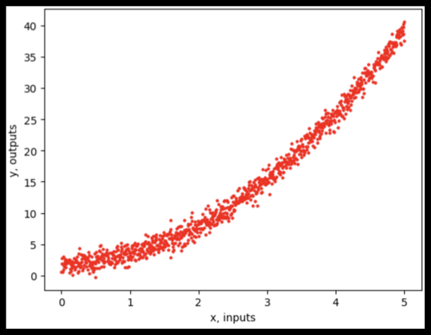
Feature engineering
# Create features
def design_matrix(x, degree):
    X = np.zeros((len(x), degree+1))
    for i in range(X.shape[1]):
        X[:, i] = x**i
    return X

degree = 2
X = design_matrix(x, degree)
y = y.reshape(-1, 1)
Shuffle and split
# Split data
n_train = int(0.8 * num_points)
n_test = num_points - n_train

shuff_index = np.random.permutation(num_points)
X_shuffle = X[shuff_index]
y_shuffle = y[shuff_index]

X_train = X_shuffle[:n_train]
X_test = X_shuffle[n_train:]
y_train = y_shuffle[:n_train]
y_test = y_shuffle[n_train:]
Visualize the split
# Plot training data
plt.plot(X_train[:, 1], y_train, 'ro', ms=2, label='Training data')
plt.plot(X_test[:, 1], y_test, 'go', ms=2, label='Test data')
plt.legend(); plt.show()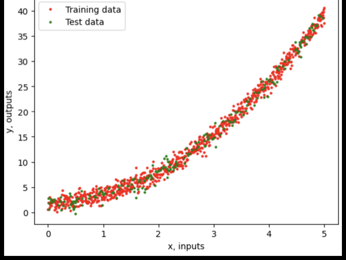
Cost function and gradient descent
Cost function
def cost_function(X, y, theta):
    m = len(y)
    return 1/(2*m) * np.sum((X @ theta - y)**2)
Run it
theta = np.random.randn(degree+1, 1)
learning_rate = 0.01
num_iters = 10000
theta, J_history = gradient_descent(
    X_train, y_train, theta,
learning_rate, num_iters)Gradient descent
def gradient_descent(X, y, theta,
                     learning_rate, num_iters):
    m = len(y)
    J_history = np.zeros(num_iters)
    for i in range(num_iters):
        theta = theta - (learning_rate/m) \
            * X.T @ (X @ theta - y)
        J_history[i] = cost_function(X, y, theta)
    return theta, J_history
Plot the result
# plot comparison
plt.plot(X_train[:, 1], y_train, 'ro', ms=2, label='Training data')
plt.plot(X_test[:, 1], y_test, 'go', ms=2, label='Test data')
plt.plot(X_train[:, 1], X_train @ theta, 'bo', ms=2, label='Model')
plt.legend(); plt.show()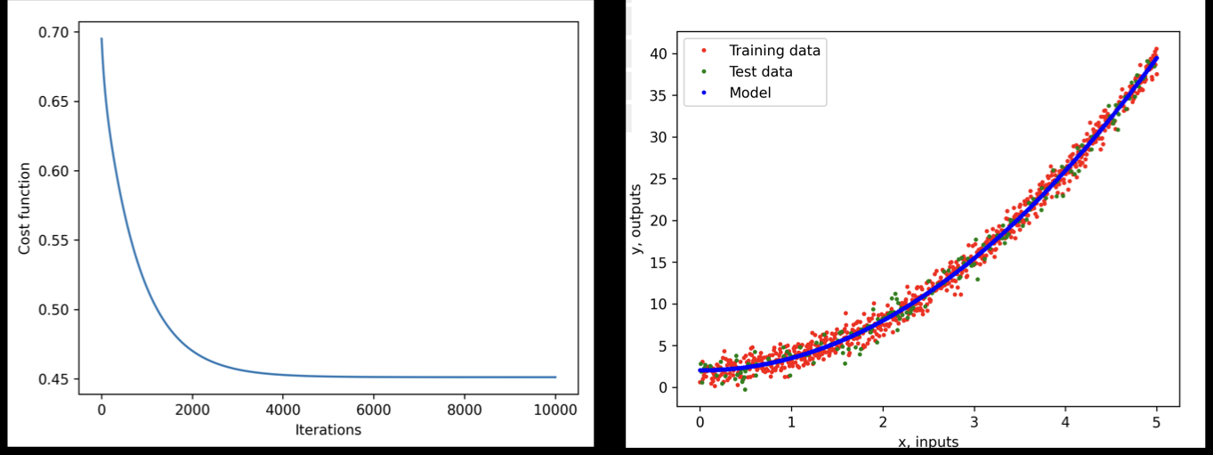
Train and test loss
test_loss  = cost_function(X_test,  y_test,  theta)
train_loss = cost_function(X_train, y_train, theta)

print(f'Test loss:  {test_loss}')
print(f'Train loss: {train_loss}')What to take away
- Training error falls as the model grows, and never warns you: the twenty houses reached $144 million off at degree 9.
- Hold data out. Choose with a validation set, or with cross validation when data are few; touch the test set once.
- Choosing is fitting: pick among many models on the test set and its score turns optimistic.
- A feature map \(\phi(x)\) lets a linear model draw curves; regularization keeps it from drawing too many.
- L2 makes coefficients smaller; L1 makes some of them exactly zero, because the diamond has corners.