Introduction to Machine Learning

Classification &
Logistic Regression

From predicting numbers to predicting labels

Given new input, what’s the output?

InputOutput
\( x^{(1)} \)\( y^{(1)} \)
\( x^{(2)} \)\( y^{(2)} \)
\( x^{(3)} \)\( y^{(3)} \)
\( x^{(4)} \)\( y^{(4)} \)
\( \vdots \)\( \vdots \)
Query  \( x_q \) ??  Prediction

Given new input, what’s the output?

Assuming \( y \in \mathbb{R} \)
\( x \)
\( \xrightarrow{\;\;h\;\;} \)
\( y \)
Given the data,
find a function \( h \),
that predicts \( y \), given \( x \)
\( \mathbf{y} = h(\mathbf{x}) \)

What if \( y \) is a label?

\( x \)
\( \xrightarrow{\;\;h\;\;} \)
\( y \)
Given the data,
find a function \( h \),
that predicts \( y \), given \( x \)
\( \mathbf{y} = h(\mathbf{x}) \)
\( y \in [0, 1] \)
A step function, or threshold
A smooth function that returns
probability of occurrence

What if \( y \) is a label?

\( y = h_\theta(x) \)&\( y \in [0,1] \)
\( y = \dfrac{1}{1 + e^{-x}} \)
Logistic function
\( h_\theta(x) = \dfrac{1}{1 + e^{-(\theta_0 + \theta_1 x)}} \)
A smooth function that returns
probability of occurrence
midpoint \( x_0 = -\theta_0/\theta_1 = \)

The curve crosses \( \tfrac12 \) where \( \theta_0 + \theta_1 x = 0 \), at \( x_0 = -\theta_0/\theta_1 \). So \( \theta_1 \) sets the steepness but also moves the midpoint; to steepen in place, scale \( \theta_0 \) with it.

What if \( y \) is a label?

\( y = h_\theta(x) \)&\( y \in [0,1] \)
\( h_\theta(x) = \dfrac{1}{1 + e^{-(\theta^\top x)}} \)
For \( x \in \mathbb{R}^n \)

Where  \( \theta^\top x = \theta_0 + \theta_1 x_1 + \theta_2 x_2 + \ldots \)

\( \theta = [\theta_0, \theta_1, \ldots] \)
\( x = [x_0, x_1, \ldots] \)
Read \( h_\theta(x) \) as \( P(y = 1 \mid x;\, \theta) \). Still a linear model at heart: the linearity lives inside \( \theta^\top x \); the sigmoid only turns that score into a probability.
A smooth function that returns
probability of occurrence

What if \( y \) is a label?

\( y = h_\theta(x) \)&\( y \in [0,1] \)
\( h_\theta(x) = \dfrac{1}{1 + e^{-(\theta^\top x)}} \)
  • 1.Define a predictor: the logistic function ✓
  • 2.Define a loss: distance between function and data ?
  • 3.Optimize loss
  • 4.Test model

The same four steps for every supervised learning algorithm.

How do we pick the best parameters \( \theta \)?

\( h_\theta(\mathbf{x}) = \theta^\top \mathbf{x} = \displaystyle\sum_{i=0}^{d} \theta_i x_i \)
Cost function
\( J(\theta) = \dfrac{1}{2} \displaystyle\sum_{i=1}^{m} \Big( h_\theta\big(x^{(i)}\big) - y^{(i)} \Big)^2 \)
\( = \dfrac{1}{2} \displaystyle\sum_{i=1}^{m} \big( \theta^\top x^{(i)} - y^{(i)} \big)^2 \)
Ordinary least squares

Logistic Regression

\( y = h_\theta(x) \)
\( h_\theta(x) = \dfrac{1}{1 + e^{-(\theta^\top x)}} = \sigma\big(\theta^\top x\big) \)
Linear predictor
negative log-likelihood or OLS
\( J(\theta) = \tfrac{1}{2} \textstyle\sum_{i=1}^{m} \big( h_\theta(x^{(i)}) - y^{(i)} \big)^2 \)
Logistic predictor
Binary cross-entropy loss
\( \begin{aligned} J(\theta) = -\textstyle\sum_{i=1}^{m} \big[ &\, y^{(i)} \log h_\theta(x^{(i)}) \\ &+ (1 - y^{(i)}) \log\big(1 - h_\theta(x^{(i)})\big) \big] \end{aligned} \)
Compute gradient \( \nabla J(\theta) \)
Gradient descent. Done!

Logistic Regression

\( y = h_\theta(x) \)
\( h_\theta(x) = \dfrac{1}{1 + e^{-(\theta^\top x)}} = \sigma\big(\theta^\top x\big) \)
Linear predictor
negative log-likelihood or OLS
\( J(\theta) = \tfrac{1}{2} \textstyle\sum_{i=1}^{m} \big( h_\theta(x^{(i)}) - y^{(i)} \big)^2 \)

Why not use an ordinary least squares loss?

✏ exercise · do it now What goes wrong if you fit the labels \( 0/1 \) by least squares?
theta = np.linalg.lstsq(X, y)[0]   # why not?

Squared Error Meets the Sigmoid

The loss as a function of \( \theta_1 \) on the tumor data. Squared error saturates into flat plateaus where the gradient dies; cross-entropy stays a clean bowl.

What Are Those Two Curves?

Write \( z = \theta^\top x \). Each example pays a per-example loss \( \ell(z) \), and
\( J(\theta) = \tfrac{1}{m}\sum_i \ell\big(\theta^\top x^{(i)}\big) \) is their average: the curves on the last slide, swept over \( \theta_1 \).

One example with \( y = 1 \), loss against the score \( z \).

Squared error
\( \begin{aligned} \ell_{\mathrm{SE}} &= (\sigma(z) - y)^2 \\ \ell_{\mathrm{SE}}'(z) &= 2\,(\sigma(z) - y)\,\sigma(z)\,(1-\sigma(z)) \end{aligned} \)
Confidently wrong means \( \sigma \approx 0 \) or \( 1 \), and the factor \( \sigma(1-\sigma) \) kills the gradient. Not convex in \( \theta \).
Cross-entropy
\( \begin{aligned} \ell_{\mathrm{CE}} &= -\big[\, y \log \sigma(z) + (1-y)\log(1-\sigma(z)) \,\big] \\ \ell_{\mathrm{CE}}'(z) &= \sigma(z) - y \end{aligned} \)
The \( \sigma(1-\sigma) \) cancels against the log's derivative, so the gradient is the error itself and never dies. Convex in \( \theta \).

The Loss Probability Chooses

Same move as last lecture: the model gives a probability for each label, so ask which \( \theta \) makes the observed labels most likely.

\( P\big(y \mid x; \theta\big) = \begin{cases} \sigma(\theta^\top x) & y = 1 \\[2pt] 1 - \sigma(\theta^\top x) & y = 0 \end{cases} \)

Both cases in one expression (check \( y = 1 \) and \( y = 0 \)), then a product over the i.i.d. examples. That product is the likelihood:

Likelihood \( L(\theta) \) \( \displaystyle L(\theta) = \prod_{i=1}^{m} P\big(y^{(i)} \mid x^{(i)}; \theta\big) = \prod_{i=1}^{m} \sigma(\theta^\top x^{(i)})^{\,y^{(i)}} \big(1 - \sigma(\theta^\top x^{(i)})\big)^{\,1-y^{(i)}} \)

The probability the model gives to the labels we actually observed, read as a function of \( \theta \) with the data fixed. Maximum likelihood picks the \( \theta \) that makes it largest.

Log, Then Average

Take \( \log \): the product becomes a sum and the exponents come down.

\( \displaystyle \log L(\theta) = \sum_{i=1}^{m} \left[ y^{(i)} \log \sigma(\theta^\top x^{(i)}) + (1 - y^{(i)}) \log \big(1 - \sigma(\theta^\top x^{(i)})\big) \right] \)

Flip the sign to get something to minimize, and average. That is the loss \( J \); each example contributes its own negative log-likelihood \( \ell^{(i)} \):

\( \displaystyle J(\theta) = -\frac{1}{m} \log L(\theta) = \frac{1}{m} \sum_{i=1}^{m} \ell^{(i)}(\theta), \qquad \ell^{(i)} = -\log P\big(y^{(i)} \mid x^{(i)}; \theta\big) \)

Notation for the rest of the course: \( L \) is the likelihood of the whole data set, \( \log L \) the log-likelihood,
\( \ell^{(i)} \) one example's loss, \( J \) the loss we minimize.

Binary Cross-Entropy

\( \displaystyle J(\theta) = -\frac{1}{m} \sum_{i=1}^{m} \left[ y^{(i)} \log \sigma(\theta^\top x^{(i)}) + (1 - y^{(i)}) \log(1 - \sigma(\theta^\top x^{(i)})) \right] \)
Reading it Only one term is active per example. Confident and right: loss near 0. Confident and wrong: \( -\log(p) \) explodes.
Why it wins Convex in \( \theta \), no dead plateaus, and it is exactly maximum likelihood for the Bernoulli model.

Your Turn: The Gradient

You have the ingredients. Same task as linear regression, new loss.

\( \displaystyle J(\theta) = -\frac{1}{m} \sum_{i=1}^{m} \left[ y^{(i)} \log \sigma(\theta^\top x^{(i)}) + (1 - y^{(i)}) \log \big(1 - \sigma(\theta^\top x^{(i)})\big) \right] \)
✏ exercise · do it now
\( \dfrac{\partial J}{\partial \theta_j} = \; ? \)

Hint: \( \sigma'(z) = \sigma(z)\big(1 - \sigma(z)\big) \), the derivative comes free. Take five minutes, then compare.

The Gradient Is an Old Friend

The sigmoid's self-derivative cancels the log's denominator, and everything collapses:

Gradient \( \displaystyle \frac{\partial J}{\partial \theta_j} = \frac{1}{m} \sum_{i=1}^{m} \left( \sigma(\theta^\top x^{(i)}) - y^{(i)} \right) x_j^{(i)} \)
Deja vu Identical in form to linear regression's gradient! Different model, and different loss, but same update rule. Is this a coincidence?

So training is unchanged: \( \theta := \theta - \frac{\alpha}{m} X^\top (\sigma(X\theta) - y) \).

Higher dimensional inputsFor Logistic Regression and beyond

\( x_1 \)\( x_2 \)\( y \)
-2-1●
31★
23●
1-1★
\( \vdots \)
\( h_\theta(x) = \dfrac{1}{1 + e^{-(\theta_0 + \theta_1 x_1 + \theta_2 x_2)}} \)
\( \theta_0 + \theta_1 x_1 + \theta_2 x_2 = 0 \)

Watch the Boundary Learn

iter 0 · J =

Two measured features (tumor size, cell irregularity). The decision boundary is \( \theta^\top x = 0 \) and the shading is \( P(y=1) \). Click inside the plot to add a malignant point and watch the boundary respond.

The Geometry of the Boundary

The boundary Predict 1 when \( P \ge \tfrac12 \), that is when the score \( \theta_0 + \theta_1 x_1 + \theta_2 x_2 \) is positive. The boundary is where the score is \( 0 \).
The normal \( (\theta_1, \theta_2) \) is perpendicular to the line and points to the positive side. \( \theta_0 \) has no direction: it only slides the line.
The distance
\( d = \dfrac{\theta_0 + \theta_1 x_1 + \theta_2 x_2}{\sqrt{\theta_1^2 + \theta_2^2}} \)
\( \theta_0 \) is not in the norm because it is not part of the direction. Further out, more confident:
\( P \to 0 \) or \( 1 \).

The Margin

Labels \( y \in \{-1, +1\} \) Relabel the classes \( \pm 1 \). Then a point is on the correct side exactly when \( y\,(\theta^\top x) > 0 \): the sign of the score agrees with the label.
Margin of one point
\( \begin{aligned} \hat\gamma^{(i)} &= y^{(i)}\,\theta^\top x^{(i)} &&\text{functional} \\ \gamma^{(i)} &= y^{(i)}\,\dfrac{\theta^\top x^{(i)}}{\lVert \theta_{1:2} \rVert} &&\text{geometric} \end{aligned} \)
The geometric margin is the signed distance of the last slide: positive for correct points, negative for mistakes.
Margin of the boundary \( \gamma = \min_i \gamma^{(i)} \): the distance to the closest point. Wider is safer; the boundary that maximises it is the support vector machine.

Step 4: Test. But Accuracy of What?

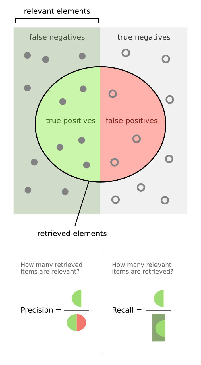
precision and recall

Every prediction lands in one of four cells: TP flagged and real, FP flagged and not, FN missed, TN correctly ignored.

Precision
\( \text{P} = \dfrac{TP}{TP + FP} \)
Of everything we flagged, how much was real.
Accuracy
\( \dfrac{TP + TN}{TP + TN + FP + FN} \)
Of everything, how much we got right.
Recall
\( \text{R} = \dfrac{TP}{TP + FN} \)
Of everything real, how much we caught.
F1
\( F_1 = \dfrac{2\,\text{P}\,\text{R}}{\text{P} + \text{R}} \)
One number when you need one: the harmonic mean of P and R.

The Same Four Numbers on One Screening

1000 people screened, 50 of them ill. The classifier flags 100: 40 who are ill and 60 who are not.

pred illpred well
ill (50)4010
well (950)60890
accuracy930 / 1000 = 0.93 precision40 / 100 = 0.40 recall40 / 50 = 0.80 F10.53
The trap Flag nobody: accuracy 0.95, better than the classifier, and recall 0. Accuracy rewards agreeing with the majority.
Which number, when Recall when a miss is the expensive error: cancer screening, fraud, a security scan.
Precision when a false alarm is the expensive error: spam filters (a real email lost), an alert a human must investigate.
Accuracy only when classes are balanced and both errors cost the same.
F1 when you must rank models by one number and care about both.

When Accuracy Lies: Imbalanced Data

pred 1pred 0
true 100
true 000
accuracy precision recall F1

Practical advice With 1% positives, predicting "no" for everyone scores 99% accuracy and catches nobody. Report precision and recall, not accuracy. Then move the threshold: lower it to buy recall when a miss is expensive (disease, fraud), raise it to buy precision when a false alarm is expensive.

Reading the Metrics Together

Tumour data with 300 more healthy patients (6% ill): one trained model, every threshold from 0 to 1.

One model, many classifiers Training fixes \( \theta \); the threshold is chosen afterwards. Lower it: recall up, precision down. Raise it: the reverse.
What accuracy is doing Past a threshold of 0.3 it sits above 0.95 and barely moves, while precision and recall swing between 0.5 and 1. It cannot see the trade, so it is the wrong compass here.
What to report Confusion matrix, precision and recall at the threshold you deploy. To compare models regardless of threshold: the precision-recall curve, or the ROC curve, and the area under it.

Logistic Regression in Twelve Lines


import numpy as np

def sigmoid(z):
    return 1.0 / (1.0 + np.exp(-z))

X = np.c_[np.ones(len(x1)), x1, x2]   # n x 3: bias + two features
theta = np.zeros(3)
alpha = 0.5

for t in range(2000):                 # batch gradient descent
    p = sigmoid(X @ theta)            # predicted probabilities
    theta -= alpha / len(y) * (X.T @ (p - y))

print(theta)                          # boundary: theta . x = 0
    

Line 12 is the whole lecture: (prediction error) times (input), averaged. Swap the sigmoid for the identity and this is last week's linear regression code. In scikit-learn the same fit is LogisticRegression().fit(X, y).

✏ exercise · do it now What is the loop doing: batch gradient descent, stochastic gradient descent, something else? What would you change to make it the other one?

Higher dimensional outputsMulti-class classification: Softmax regression

\( \mathbf{x} \)
\( \mathbf{y} = h_\theta(\mathbf{x}) \) \( \xrightarrow{\qquad\quad} \)
\( \mathbf{y} \)

\( k \) discrete values for representing output \( \mathbf{y} \)

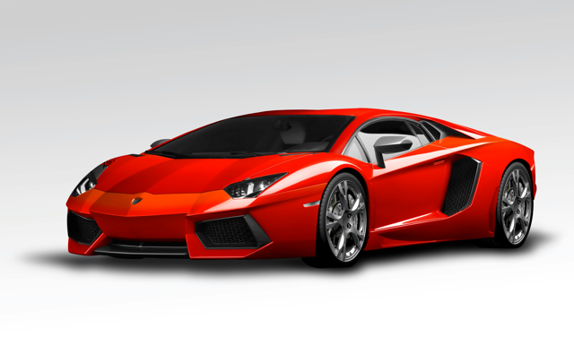
car
\( \begin{bmatrix} 1 \\ 0 \\ 0 \\ 0 \end{bmatrix} \)
car
plane
\( \begin{bmatrix} 0 \\ 1 \\ 0 \\ 0 \end{bmatrix} \)
plane
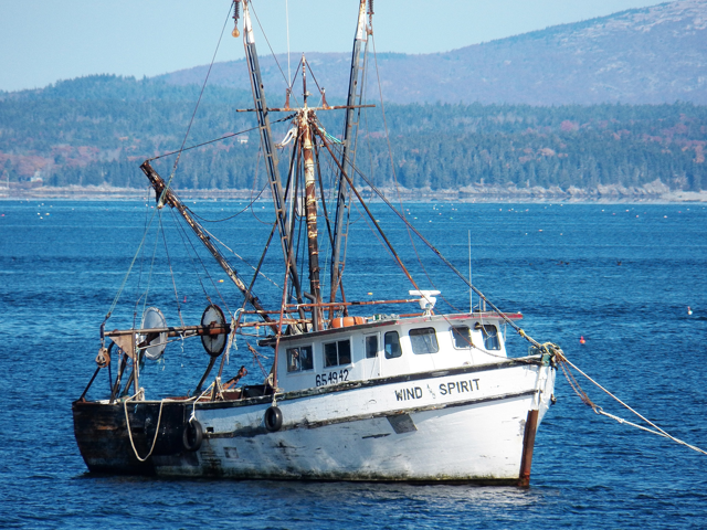
boat
\( \begin{bmatrix} 0 \\ 0 \\ 1 \\ 0 \end{bmatrix} \)
boat
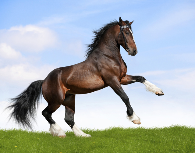
horse
\( \begin{bmatrix} 0 \\ 0 \\ 0 \\ 1 \end{bmatrix} \)
horse

One-hot encoding

How to turn scores into probabilities?Note: this slide explains the intuition. Softmax regression is not exactly equivalent to a combination of one-vs-all classifiers.

What’s the probability it’s a car? query car
WARNING!!!
Notation Alert
\( \vec{\theta}_i \) is a vector
Score
\( \vec{\theta}_1^{\top} \hat{x} = 3 \)
\( \vec{\theta}_2^{\top} \hat{x} = -0.3 \)
\( \vec{\theta}_3^{\top} \hat{x} = -0.8 \)
\( \vec{\theta}_4^{\top} \hat{x} = -22 \)
⟶
exp
Positive measure
\( \exp(3) = 20.1 \)
\( \exp(-0.3) = 0.74 \)
\( \exp(-0.8) = 0.45 \)
\( \exp(-22) = 0.00\ldots 1 \)
⟶
Normalize
Softmax
\( \hat{p}(y = i \mid x; \theta) = \dfrac{\exp\big(\vec{\theta}_i^{\top} x\big)}{\sum_{j=1}^{k} \exp\big(\vec{\theta}_j^{\top} x\big)} \)

How to turn scores into probabilities?

What’s the probability it’s a car? query car
WARNING!!!
Notation Alert
\( \vec{\theta}_i \) is a vector
Softmax
\( \hat{p}(y = i \mid x; \theta) = \dfrac{\exp\big(\vec{\theta}_i^{\top} x\big)}{\sum_{j=1}^{k} \exp\big(\vec{\theta}_j^{\top} x\big)} \)
\( \hat{p}_\Theta = \begin{bmatrix} \hat{p}(y = \text{car} \mid x; \theta_1) \\ \hat{p}(y = \text{plane} \mid x; \theta_2) \\ \hat{p}(y = \text{boat} \mid x; \theta_3) \\ \hat{p}(y = \text{horse} \mid x; \theta_4) \end{bmatrix} \)
\( \hat{p}_\Theta = \mathrm{Softmax}(\Theta x) \)

How do you train?

Given label
\( \begin{bmatrix} 1 \\ 0 \\ 0 \\ 0 \end{bmatrix} \)
car
Prediction
WARNING!!!
\( y \) is the
ground-truth index
\( \underset{\vec{\theta}_1, \vec{\theta}_2, \vec{\theta}_3, \vec{\theta}_4}{\operatorname{argmin}} \)
\( \mathrm{CrossEntropy}(p, \hat{p}) = -\displaystyle\sum_{i=1}^{k} p(y = i)\, \log\big(\hat{p}(y = i)\big) \)
\( = -\log\big(\hat{p}(y = 1)\big) \)

How do you train?

Prediction
\( \mathrm{CrossEntropy}(p, \hat{p}) = -\displaystyle\sum_{i=1}^{k} p(y = i)\, \log\big(\hat{p}(y = i)\big) \)
Logit \( = -\log\big(\hat{p}(\colorbox{#d19a66}{$y$} = 1)\big) \)
\( = -\log\left( \dfrac{\exp\big(\vec{\theta}_y^{\top} x\big)}{\sum_{j=1}^{k} \exp\big(\vec{\theta}_j^{\top} x\big)} \right) \)

The logit is the score \( \vec{\theta}_i^{\top} x \) inside the exponential; the softmax turns logits into probabilities.

Train with Gradient Descent!

Explore Further

Some useful reference interactive websites:

They open inside the slide; press Esc to come back.

Look closely The Playground link has zero hidden layers and a sigmoid output. That configuration is logistic regression: one neuron. Hold that thought for two lectures.

What if the boundary needs to curve?

No straight line separates these classes. Two answers exist: invent better features by hand, or let the model learn them. That second answer is called a neural network.

Summary

The model
\( P(y{=}1 \mid x) = h_\theta(x) = \sigma(\theta^\top x) \)

a linear score squashed to a probability

The loss
\( J(\theta) = -\tfrac{1}{m}\sum_i \big[ y \log \sigma + (1{-}y)\log(1{-}\sigma) \big] \)

maximum likelihood for Bernoulli labels; convex

The update
\( \theta := \theta - \tfrac{\alpha}{m} X^\top(\sigma(X\theta) - y) \)

error times input, again

Many classes
\( \hat{p}_\Theta = \mathrm{Softmax}(\Theta x) \)

one-hot labels, one score per class, cross-entropy loss

Caveats: boundaries are straight; accuracy misleads when classes are imbalanced; pick the threshold for the cost you care about. Next: maximum likelihood as a worldview, and the family that unites linear and logistic regression.