Introduction to Machine Learning
Generative Learning
and Language
From counting words to predicting the next one
Five questions for today
- 1Words as dataHow does a message become numbers?
- 2Count, then flipHow do you classify by counting?
- 3Model each classWhat if you modeled what each class looks like?
- 4Generating languageWhat does it take to write the next word?
- 5In codeWhat does Naive Bayes look like in fifteen lines?
Three real datasets: 5,574 text messages people actually received, the Palmer penguins from the data lecture, and a whole book, Gibran's The Prophet.
Spam vs Not Spam
A classifier reads the words and decides. But a message is not a number, so what is \(x\)?
5,574 real text messagesThe SMS Spam Collection, labelled by hand
Short, misspelled, full of "u" and "2" and "lor": this is language as people use it. Every model today is trained on four fifths of these messages and tested on the rest (every fifth message), which it never sees.
Data: Almeida, Gómez Hidalgo and Yamakami, Contributions to the study of SMS spam filtering, DocEng 2011, via the UCI repository (CC BY 4.0). Messages shown are drawn at random.
Language: One-Hot Word Representation
Bag of Words
Drop the order. Ask only: is this word present? Define \( x_j = 1 \) or \( x_j = 0 \).
Each email is now a row of zeros and ones, and a label \(y\): the same table shape we have used since week one.
Part 2 of 5
Count, then flip
How do you classify by counting?
What Are the Relevant Probabilities?
counted from the six emails above
The Naive Assumption
We want the probability of a whole message, not one word:
There are \(2^n\) possible messages, so we can never count them all. Assume the words are conditionally independent given the label:
It is wrong: "prize" and "win" travel together. It is also enough, which is the useful kind of wrong.
Bayes Rule Turns It Around
We can count \( P(x \mid y) \). What we want is \( P(y \mid x) \).
For a Given Dataset
\( \{ (x^{(i)}, y^{(i)}) \}_{i=1}^{M} \), estimate each piece by counting.
That is the whole training procedure: count, divide, store. No gradient descent anywhere.
Naming the parameters: \(\phi\)Every probability the model needs is one number to learn
| Parameter | What it means | From the training messages |
|---|---|---|
| \( \phi_y = P(y = 1) \) | the share of messages that are spam | \( 591 / 4{,}459 = 0.133 \) |
| \( \phi_{j \mid y=1} = P(x_j = 1 \mid y = 1) \) | the chance a spam message contains word \(j\) | call: \( 265 / 591 = 0.448 \) |
| \( \phi_{j \mid y=0} = P(x_j = 1 \mid y = 0) \) | the chance a normal message contains word \(j\) | call: \( 180 / 3{,}868 = 0.047 \) |
Each \(\phi\) is the probability of a coin landing heads, so it lies between 0 and 1. The model is \(1 + 2n\) such coins: 15,989 numbers for a dictionary of 7,994 words.
A message's probability is then a product of coins, heads for each word present and tails for each word absent:
\(y \in \{0, 1\}\): the label, 1 for spam.
\(j = 1, \dots, n\): a word of the dictionary; here \(n = 7{,}994\).
\(x_j \in \{0, 1\}\): 1 if word \(j\) appears in the message.
\(x^{(i)}, y^{(i)}\): the \(i\)-th training message and its label, \(i = 1, \dots, M\); here \(M = 4{,}459\).
\(\phi\): Greek "phi", the usual name for a probability that is a parameter.
Finding \(\phi\): maximum likelihood is countingWhy the formulas on "For a Given Dataset" are the best possible values
1. The likelihood of the training set is the probability the model gives to everything we saw:
2. Take the log. The product becomes a sum, and the sum splits into separate pieces: each \(\phi\) appears in exactly one piece, so each can be found on its own.
3. Each piece is a coin. For \(\phi_{j \mid y=1}\): of the \(M_1\) spam messages, \(a\) contain word \(j\) and \(b = M_1 - a\) do not. Its piece is
4. Set the slope to zero: \( \dfrac{a}{\phi} - \dfrac{b}{1 - \phi} = 0 \;\Longrightarrow\; \phi = \dfrac{a}{a + b} = \dfrac{a}{M_1} \).
\( \phi_{j \mid y=1} = \dfrac{\text{spam messages containing word } j}{\text{spam messages}} \)
For "call": \(a = 265\), \(b = 326\), so \(\phi = 265 / 591 = 0.448\). No value of \(\phi\) makes the training messages more probable.
The same steps give \(\phi_y = 591 / 4{,}459\), and in Part 3 the GDA parameters: \(\phi\), the means \(\mu_k\), the covariance \(\Sigma\). It is the coin of the maximum likelihood lecture, once per word.
Laplace smoothing ("The word it never saw") adds imaginary sightings to the counts: \( (a + 1) / (M_1 + 2) \).
Every word casts a voteType a message. The filter is trained on 4,459 real ones.
\(x_t\) is the \(t\)-th of the \(d\) words of the message \(x\), repeats included; \(P(x_t \mid y)\) is how often that word occurs among the training words of class \(y\), counted on the next slide. Why a ratio, and why logs: the deep dive after this slide.
Try "a real prize": a friend's message, flagged as spam, because "won" and "prize" have only ever appeared in spam. The filter is right about its data and wrong about your friend.
Where the vote comes fromFrom Bayes' rule to a sum of bars, on the message "Congratulations! You won a prize, call now to claim"
1. Bayes for both labels. \( P(\text{spam} \mid x) = \dfrac{P(x \mid \text{spam})\, P(\text{spam})}{P(x)} \), and the same for not spam.
2. Divide them. The evidence \(P(x)\) cancels, and we never need it:
3. The naive assumption makes each likelihood a product over the words, \( P(x \mid y) = \prod_{t=1}^{d} P(x_t \mid y) \), so the ratio of products is a product of ratios.
4. Take logs. The product becomes a sum: one term per word, one bar per term. The sum of the word terms is the difference of the total log-likelihoods, \( \log P(x \mid \text{spam}) - \log P(x \mid \text{not}) \).
5. Back to a probability. \( P(\text{spam} \mid x) = \sigma(\text{log odds}) = 1 / (1 + e^{-\text{log odds}}) \): the sigmoid of logistic regression. Naive Bayes is a linear classifier in the word counts, a point Part 3 comes back to.
| term | in spam | in not spam | log ratio |
|---|---|---|---|
| prior: 591 spam, 3,868 not | −1.88 | ||
| congratulations | 11 | 1 | +2.81 |
| you | 235 | 1,494 | −0.82 |
| won | 61 | 0 | +5.15 |
| a | 293 | 865 | −0.06 |
| prize | 79 | 0 | +5.40 |
| call | 288 | 191 | +1.43 |
| now | 165 | 240 | +0.65 |
| to | 561 | 1,261 | +0.21 |
| claim | 89 | 0 | +5.52 |
| log odds | +18.42 |
Counts are occurrences among the 14,916 spam and 55,654 normal training words; each ratio uses \(\alpha = 1\). For example, \(P(\text{call} \mid \text{spam}) = 289 / 22{,}910 = 0.0126\) and \(P(\text{call} \mid \text{not}) = 192 / 63{,}648 = 0.0030\), so the term is \(\log(0.0126 / 0.0030) = +1.43\). Then \(\sigma(18.42) > 0.9999999\).
The word it never sawCounting gives zero, and zero ruins a product
\(x_t\): a word of a message; \(k\): a word of the dictionary \(V\) (7,994 words); \(y\): the label. \(\phi_{k \mid y}\): the chance a word of a class-\(y\) message is \(k\), the word-counting cousin of \(\phi_{j \mid y}\). \(\text{count}(k, y)\): times \(k\) occurs in class-\(y\) training messages; \(\text{count}(y)\): all their words (14,916 spam, 55,654 not). \(\alpha\): imaginary sightings. This is the multinomial model of the next slide.
Add \(\alpha\) imaginary sightings of every word. Maximum likelihood says "never seen, so impossible"; smoothing says "never seen, so rare". A finite sample is not proof that something cannot happen.
Two ways to generate an emailTwo event models: two stories of how a message gets written
| On the 1,115 held-out messages | accuracy | spam missed (of 156) | normal messages flagged |
|---|---|---|---|
| always "not spam" | 86.0% | 156 | 0 |
| Bernoulli Naive Bayes | 97.4% | 29 | 0 |
| multinomial Naive Bayes | 98.5% | 12 | 5 |
Neither is best at everything: the Bernoulli model never flags a friend, and lets more spam through. Which mistake is worse is a decision, not a statistic (see the logistic regression lecture).
Bernoulli or multinomial, in detailThe same messages, two different random experiments
| Multivariate Bernoulli | Multinomial | |
|---|---|---|
| A message is | \( x \in \{0, 1\}^{\lvert V \rvert} \): \(x_j = 1\) if dictionary word \(j\) appears, at least once | \( x = (x_1, \dots, x_d) \): \(x_t\) is the \(t\)-th word, \(d\) the length |
| How it is generated | for each of the \(\lvert V \rvert\) dictionary words, flip its own coin: in, or out | roll one \(\lvert V \rvert\)-sided die \(d\) times, one word per roll |
| Likelihood \(P(x \mid y)\) | \( \prod_{j=1}^{\lvert V \rvert} \phi_{j \mid y}^{\,x_j} (1 - \phi_{j \mid y})^{1 - x_j} \) | \( \prod_{t=1}^{d} \phi_{x_t \mid y} \) |
| A parameter means | \( \phi_{j \mid y} \): the chance a message of class \(y\) contains word \(j\) | \( \phi_{k \mid y} \): the share of class \(y\)'s words that are word \(k\); they sum to 1 |
| Estimated (Laplace) | \( \dfrac{\#\,\text{messages of class } y \text{ containing } j + 1}{\#\,\text{messages of class } y + 2} \) | \( \dfrac{\#\,\text{occurrences of } k \text{ in class } y + 1}{\#\,\text{words in class } y + \lvert V \rvert} \) |
| "call call call" | the same as "call": repeats are invisible | three factors of \(\phi_{\text{call} \mid y}\): repeats count |
| Words not in the message | count: every absent word multiplies in \(1 - \phi_{j \mid y}\) | ignored: only the words that occur |
Rule of thumb: presence is the signal in short texts, frequency in long documents, which is why the multinomial is the usual default for text. In these messages 1,964 of 4,459 repeat some word, and the multinomial catches more spam (the table on the last slide).
Part 3 of 5
Model each class
What if you modeled what each class looks like?
Generative and Discriminative
logistic regression
naive Bayes, Gaussian discriminant analysis
A Gaussian in two dimensionsShape it: two spreads and a correlation
The diagonal of \(\Sigma\) holds the two variances; the off-diagonal entry, \(\rho\,\sigma_1 \sigma_2\), tilts the cloud. The rings are one and two standard deviations.
Gaussian discriminant analysis, on penguinsAdelie and Chinstrap, by their bills (the data lecture's penguins)
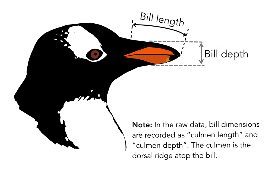

Bill length: along the top ridge. Bill depth: its height. Adelie is \(y = 0\), Chinstrap \(y = 1\); no Gentoo today. Artwork by @allison_horst.
\( x \mid y = 0 \sim \mathcal{N}(\mu_0, \Sigma) \)
\( x \mid y = 1 \sim \mathcal{N}(\mu_1, \Sigma) \)
Fitting is counting again: \(\phi\) is the share of Chinstraps, \(\mu_k\) the average bill of each species, \(\Sigma\) the spread around those averages.
Hidden inside GDA: a logistic regression
Apply Bayes rule to the GDA model and simplify. With a shared \(\Sigma\), the quadratic terms cancel:
A stronger assumption learns faster...while it holds
GDA spends its assumption as information: it only has to learn two averages and one spread. Logistic regression learns the boundary from the points near it, and needs more of them.
Part 4 of 5
Generating language
What does it take to write the next word?
Auto-Regressive Language Models
Same counting idea, one step further: predict the next word.
The context is too long to count, so an n-gram model truncates it:
An n-gram model of The ProphetKahlil Gibran, 1923: 13,000 words, learned by counting
Longer context makes it fluent, then makes it a copier: with one book there are too few examples of each long context to count anything but the original. This is the overfitting of the generalization lecture, in words. A large language model learns from far more text, and approximates the counts instead of storing them.
Text: The Prophet, Project Gutenberg eBook 58585, public domain.
Large Language Models
- An LLM is also a probabilistic model for \( P(x_1, \dots, x_n) \)
- It approximates \( P(x_i \mid x_{i-k}, \dots, x_{i-1}) \), which is \(V^k\) dimensional, instead of counting it, where \(V\) is the size of the dictionary
- The embedding replaces the one-hot vector: \( x \in \mathbb{R}^d \) instead of a \(V\)-dimensional spike
Part 5 of 5
In code
What does Naive Bayes look like in fifteen lines?
Naive Bayes from scratchPress Run: real Python, on the 5,574 messages
import numpy as np, pandas as pd, re
from collections import Counter

sms = pd.read_csv('sms_spam.csv')
words = lambda s: re.findall(r"[a-z0-9']+", s.lower())
test = sms.index % 5 == 0                      # every fifth message is held out
train = sms[~test]

counts = {c: Counter(w for s in train.text[train.label == c] for w in words(s)) for c in ('spam', 'ham')}
vocab = set(counts['spam']) | set(counts['ham'])
total = {c: sum(counts[c].values()) for c in counts}
prior = {c: np.log((train.label == c).mean()) for c in counts}

def log_p(msg, c, alpha=1):                    # count, divide, store: that was training
    return prior[c] + sum(np.log((counts[c][w] + alpha) / (total[c] + alpha * len(vocab))) for w in words(msg) if w in vocab)

guess = [max(('spam', 'ham'), key=lambda c: log_p(m, c)) for m in sms.text[test]]
print('held-out accuracy:', np.mean(np.array(guess) == sms.label[test].values).round(4))
print('most spammy words:', sorted(vocab, key=lambda w: (counts['spam'][w] + 1) / (counts['ham'][w] + 1))[-8:])
print(log_p('Free entry! Text WIN to claim', 'spam') > log_p('Free entry! Text WIN to claim', 'ham'))
You should get 0.9848, the multinomial row of the table, and a spam list ending in 'won', 'prize', 'claim'. Try alpha=0 in log_p, and a message with a word only one class has seen.
Summary
one-hot per word, then a bag of words
drops the order and keeps presence
wrong but useful, and trained by counting
turns what we can count into what we want
an n-gram counts the next word;
an LLM approximates the same probability
What to take away
- A discriminative model learns \(P(y \mid x)\). A generative one learns \(P(x \mid y)\) and \(P(y)\), then flips them with Bayes rule, and can draw new examples.
- Naive Bayes trains by counting. Its assumption is false, words travel together, and it still catches 144 of 156 spam messages it never saw.
- Zero counts are not impossibilities: Laplace smoothing adds imaginary sightings so one unseen word cannot decide everything.
- GDA models each class as a Gaussian cloud; with a shared \(\Sigma\) its posterior is exactly a logistic regression. It learns faster from little data, and breaks when the clouds are not Gaussian.
- An n-gram model writes by counting what came next. More context makes it fluent, then makes it copy: overfitting, in words.