Introduction to Machine Learning
Introduction to
Neural Networks
What if the model could invent its own features?
Seven questions for today
- 1Where the neuron came fromWhy did anyone think a network of simple units could compute?
- 2The feature problemWhat if the model could choose its own features?
- 3NetworksWhat does a stack of layers buy?
- 4TrainingHow are thousands of weights found?
- 5In codeWhat does a network look like in numpy, and in PyTorch?
- 6Real handwritingWhat does a network learn from real digits, and where does it fail?
- 7Beyond pixels as a listWhat structure in the data does a plain layer ignore?
The toy problems show the idea, and how the weights are found. Then 20,000 real handwritten digits show what a trained network learns and where it fails.
Why does deep learning work?Two principles its success reveals
Intelligence can emerge from simple elements that learn to coordinate. No single unit knows what a digit is.
Letting a system learn from its environment is more powerful than writing down its rules.
A deep network is a collection of simple elements that collaborate to turn inputs into predictions. Its power is not in any one of them but in how they adapt, together, to data.
Rules, or the ability to learn?
- Encode expert knowledge as explicit rules
- Say what to do in each situation
- Brittle when the environment changes
- Cannot adapt to contexts nobody foresaw
- Give the system the ability to learn
- Let it adapt to its environment
- Flexible where the world is unpredictable
- Stronger when you cannot list every case
Do you teach your children a rule for every situation, or the ability to adapt to any situation they meet?
The intellectual milieu of the 1940sThree ideas met
- Russell and Whitehead, Principia Mathematica (1910 to 1913): mathematics can be derived from formal logic.
- Von Neumann designed the stored-program computer (EDVAC, 1945), with McCulloch-Pitts neurons as its conceptual model.
- Norbert Wiener founded cybernetics (1948): feedback, control and communication in animals and machines.
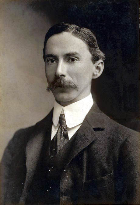
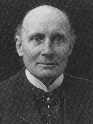
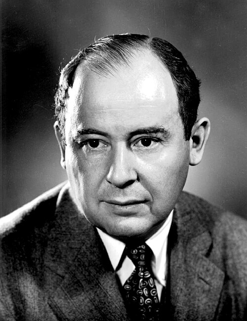
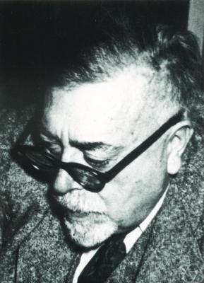
Photos: Wikimedia Commons. Russell and Whitehead public domain; von Neumann, Los Alamos National Laboratory; Wiener, Konrad Jacobs, CC BY-SA 2.0 de.
Walter Pitts and the dream of logical intelligence
Pitts was a self-taught, homeless teenager in Detroit who, at twelve, found errors in Principia Mathematica and wrote to Russell, who invited him to study with him.
He met Warren McCulloch, a neurophysiologist asking how the brain computes. Together they joined propositional logic to neural anatomy in the first formal model of a neuron.
Their 1943 paper showed that networks of binary threshold units can implement any logical function: a founding text of both neural networks and the theory of digital computers.
McCulloch chaired meetings with von Neumann, Wiener, Pitts, Bateson and Margaret Mead, where cybernetics took shape and the ideas that became AI, information theory and cognitive science were argued over.
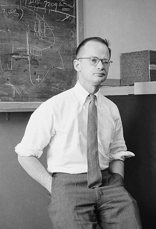
Photo: Francis Bello, public domain (Wikimedia Commons).
The McCulloch-Pitts neuron (1943)A weighted vote against a threshold. Click the inputs, pick a gate.
Weights \(\theta_i\), as in linear regression, and a threshold \(T\). With the right weights one unit is an AND, an OR, a NAND or a NOR gate. NAND alone builds any logic circuit, so networks of these units can compute anything a computer can.
What it lacks: a way to find the weights. Every one was set by hand. The rest of today is about letting data set them.
McCulloch and Pitts, A logical calculus of the ideas immanent in nervous activity, Bulletin of Mathematical Biophysics 5, 115 to 133, 1943. doi:10.1007/BF02478259
How close to a real neuron?
While McCulloch and Pitts made the neuron a logical abstraction, experimentalists measured the real thing. The squid's giant axon, up to a millimetre across, is wide enough to put an electrode inside.
- 1939: Cole and Curtis develop the voltage clamp: hold the membrane potential fixed, measure the current.
- 1952: Hodgkin and Huxley fit differential equations to voltage-clamp data, with gating variables \(m, h, n\) following first-order kinetics.
- 1963: Nobel Prize for Hodgkin, Huxley and Eccles.
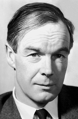
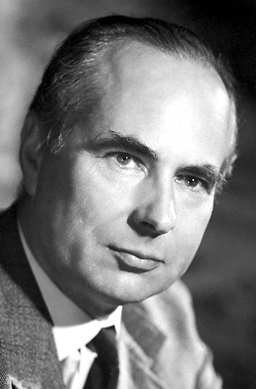
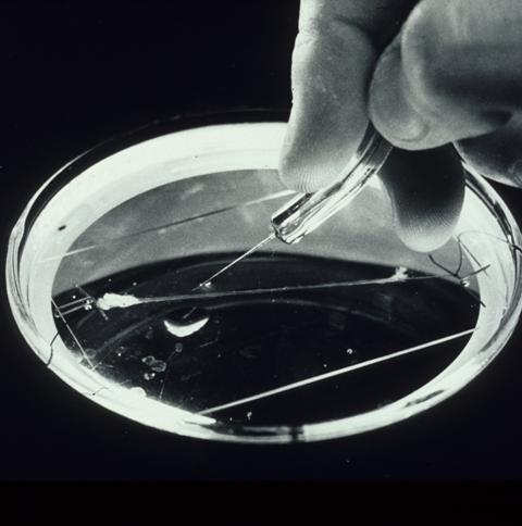
Photos: Wikimedia Commons, public domain (Hodgkin and Huxley, Nobel portraits 1963; the axon, NIH History Office).
The Hodgkin-Huxley modelFour coupled differential equations, fit to experiment
The gating variables \(m, h, n \in [0, 1]\) are the probabilities that ion-channel gates are open: sodium needs three activation gates (\(m^3\)) and one inactivation gate (\(h\)), potassium four (\(n^4\)). Each follows
with rate functions \(\alpha_x, \beta_x\) fit to the data. Raise the current: below a threshold nothing happens; above it the neuron fires, again and again.
Two views of the neuron
| McCulloch-Pitts (1943) | Hodgkin-Huxley (1952) | |
|---|---|---|
| Nature | Computational, logical | Dynamical, physical |
| Output | Binary: 0 or 1 | A continuous voltage \(V(t)\) |
| Time | Instantaneous | Evolves by coupled ODEs |
| Parameters | Weights \(\theta_i\), threshold \(T\) | Conductances, reversal potentials, gating rates |
| Found by | Construction, from logic | Fitting voltage-clamp experiments |
| Legacy | Neural networks, deep learning, AI | Computational neuroscience, biophysics |
Deep learning descends from the first column: simplified units whose power comes from collective adaptation, not biological fidelity. What matters is less the unit than the ability to learn.
Part 2 of 7
The feature problem
What if the model could choose its own features?
The ML workflowEverything so far, in one loop
Go back and choose other features, or turn the knobs: the learning rate \(\eta\), the regularization \(\lambda\), the number of iterations \(T\). These are hyperparameters.
Report \(\mathcal{L}_{\text{test}}\), once, on data the loop never touched.
The step that needs a human is the second one. How do I choose the feature vector?
The Question That Haunts Every Model
Linear and logistic regression both start the same way: someone chooses the features \( \varphi(x) = [1, x, \, ?] \). Choose well and life is easy. Choose badly and no amount of fitting saves you.
Same data, same least squares; only the feature map changes. The third one nails it, but only because we peeked at the answer.
Is it a boat?A classifier on features is a boundary: \(\varphi(x) \cdot \mathbf{\theta} = 0\)

To a linear classifier the photo is a point \(\varphi(x)\), and the answer is which side of the plane \(\varphi(x) \cdot \mathbf{\theta} = 0\) it falls on.
But which numbers should \(\varphi\) compute from a million pixels? Hull edges, the colour of water, a white shape on blue? Nobody can write that list down.
A neural network learns \(\varphi\) and \(\mathbf{\theta}\) together.
The Linear Predictor, Drawn
Take last month's model and draw it as a circuit: inputs flow in, get weighted, get summed.
\( f_{\mathbf{w}}(x) \;=\; w_1 x_1 + w_2 x_2 + w_3 x_3 \;=\; \mathbf{w} \cdot \mathbf{x} \)
Two Outputs Make a Matrix
\( \hat y_1 = \mathbf{w}_1 \cdot \mathbf{x} = w_{11}x_1 + w_{12}x_2 + w_{13}x_3 \)
\( \hat y_2 = \mathbf{w}_2 \cdot \mathbf{x} = w_{21}x_1 + w_{22}x_2 + w_{23}x_3 \)
3 × 2 fitting parameters, one per arrow
Index notation, the bias, the dimensions
Each output is a weighted sum of every input, plus its own offset:
\(n\) inputs, \(m\) outputs: \(\mathbf{W}\) has one row per output and one column per input, so \(mn\) weights and \(m\) biases.
Some books write \(\mathbf{b}\) explicitly; others add \(x_0 = 1\) to \(\mathbf{x}\) and hide \(\mathbf{b}\) in \(\mathbf{W}\). Same model. The pictures from here on leave \(\mathbf{b}\) out, for clarity only.
The Nonlinear Predictor
The Activation Menu
Solid: the function. Dashed: its derivative, which is what training will care about. Watch where the derivative dies; flat derivative means no learning signal.
Part 3 of 7
Networks
What does a stack of layers buy?
Neural Network
nonlinear ∘ linear ∘ nonlinear ∘ linear
Going deepStack layers: every hidden layer is a feature map of the one before
Widths can differ from layer to layer: here 3 inputs, 2 hidden units, then 4, then 2 outputs. \(\mathbf{W}_2\) is 4 by 2.
One notation for every layer\(\mathbf{z}\) before the squash, \(\mathbf{v}\) after, \([l]\) for the layer

flatten the pixels into \(\mathbf{x}\), push them through three layers, read "cat" from \(\hat y = v^{[3]}\)
In general \(\mathbf{z}^{[l]} = \mathbf{W}^{[l]}\mathbf{v}^{[l-1]} + \mathbf{b}^{[l]}\) and \(\mathbf{v}^{[l]} = \sigma(\mathbf{z}^{[l]})\), with \(\mathbf{v}^{[0]} = \mathbf{x}\). The whole network is the hypothesis \(\hat y = f_{\mathbf{W}^{[1]}\mathbf{W}^{[2]}\mathbf{W}^{[3]}}(\mathbf{x})\). Part 6 differentiates it.
The Problem a Line Cannot Solve
The XOR arrangement from the lecture. Train the one-neuron model and watch it give up; switch to the tiny network and watch the boundary bend.
How Expressive Is One Hidden Layer?
Then Why Go Deep?
The Recipe Survives, the Landscape Does Not
Same four steps as always: predictor, loss, optimize, test. One thing breaks quietly:
Why deep learning? Feature learning\(\varphi_1(\mathbf{x})\), then \(\varphi_2(\varphi_1(\mathbf{x}))\), then \(\varphi_3(\varphi_2(\varphi_1(\mathbf{x})))\)
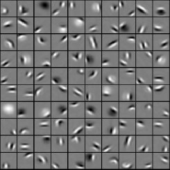
layer 1: edges
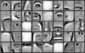
layer 2: parts of faces
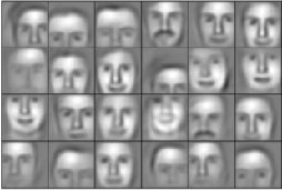
layer 3: faces
Features a network learned from face images, layer by layer, with no one telling it what an eye is. Each layer builds its features out of the features below.
Lee, Grosse, Ranganath and Ng, Unsupervised learning of hierarchical representations with convolutional deep belief networks, Communications of the ACM 54(10), 2011. doi:10.1145/2001269.2001295
Part 4 of 7
Training
How are thousands of weights found?
Six thousand knobs. Who turns them?
Gradient descent needs the gradient of the loss with respect to every weight, through every layer. The chain rule becomes an algorithm, and the algorithm is called backpropagation.
The loss, and the approachThe recipe you know, with a network as the hypothesis
The negative log-likelihood of a Bernoulli, exactly as in logistic regression and the GLM lecture.
Training loss \( \displaystyle \mathcal{L}(\mathbf{W}_1, \mathbf{W}_2) = \frac{1}{n} \sum_{i=1}^{n} \ell\big(\mathbf{x}^{(i)}, \mathbf{y}^{(i)}; \mathbf{W}_1, \mathbf{W}_2\big) \)
Objective \( \displaystyle \hat{\mathbf{W}}_1, \hat{\mathbf{W}}_2 = \arg\min_{\mathbf{W}_1, \mathbf{W}_2} \mathcal{L}(\mathbf{W}_1, \mathbf{W}_2) \)
Optimal predictor \( f_{\hat{\mathbf{W}}_1 \hat{\mathbf{W}}_2}(\mathbf{x}) = \hat{\mathbf{W}}_2\, \sigma(\hat{\mathbf{W}}_1 \mathbf{x}) \)
No normal equations this time: the minimum has no closed form. Gradient descent it is.
Gradient descent on a landscape that is not a bowl
A made-up two-weight loss, dark where it is low. Click anywhere to start there. From some starts you reach the deepest valley, from others a shallower one; too large an \(\alpha\) and you bounce.
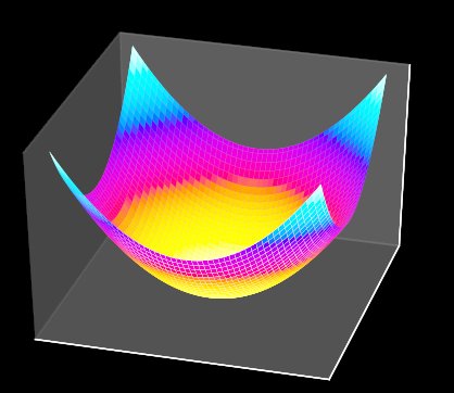
linear model: one bowl
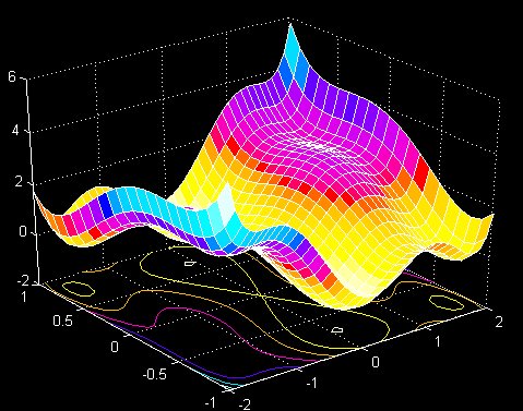
network: many valleys
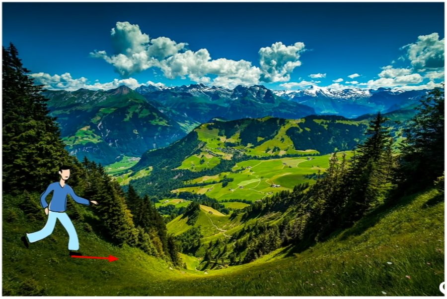
you only see the slope under your feet
Update every layerSo we need \(\partial \mathcal{L} / \partial \mathbf{W}^{[i]}\) and \(\partial \mathcal{L} / \partial \mathbf{b}^{[i]}\) for every layer
The chain rule, following the hypothesis from the loss back to each weight:
\( \mathbf{z}^{[1]} = \mathbf{W}^{[1]}\mathbf{x} + \mathbf{b}^{[1]} \)
\( \mathbf{v}^{[1]} = \sigma(\mathbf{z}^{[1]}) \)
\( \mathbf{z}^{[2]} = \mathbf{W}^{[2]}\mathbf{v}^{[1]} + \mathbf{b}^{[2]} \)
\( \mathbf{v}^{[2]} = \sigma(\mathbf{z}^{[2]}) \)
\( z^{[3]} = \mathbf{W}^{[3]}\mathbf{v}^{[2]} + b^{[3]} \)
\( \hat y = \sigma(z^{[3]}) \)
The last layer, by handSigmoid output, cross-entropy loss, one example
Multiply the first two: \( \big(-\tfrac{y}{\hat y} + \tfrac{1-y}{1-\hat y}\big)\, \hat y (1-\hat y) = -y(1-\hat y) + (1-y)\hat y = \hat y - y \). The sigmoid's derivative cancels the loss's denominators.
The error times what came in: the same form as the logistic regression gradient, with \(\mathbf{v}^{[2]}\) in place of \(\mathbf{x}\). Then \( \mathbf{W}^{[3]} \leftarrow \mathbf{W}^{[3]} - \alpha (\hat y - y)\, \mathbf{v}^{[2]\top} \).
The products share their beginnings
The boxed factor is common to every gradient below the output layer, and the next factors are common to everything below layer 2.
Can we save each product once, and reuse it for all the gradients below it? That is backpropagation.
Computation graphsEvery formula is a graph of small operations; each knows its local derivatives
You built this in the Math and Python deck: the chain rule, as a picture, and backpropagation in twenty lines.
The chain rule on a graphWalk back along the path and multiply the local derivatives
Backpropagation, step by stepOne weight, one example: values flow forward, derivatives flow back. Press Forward, then Backward.
A two-layer network as a graph\( \mathcal{L} = \lVert \sigma(\mathbf{W}_2\, \sigma(\mathbf{W}_1 \mathbf{x})) - \mathbf{y} \rVert^2 \), with \(\sigma(x) = 1/(1 + e^{-x})\)
Forward, top to bottom: \(\mathbf{s}_1 = \mathbf{W}_1 \mathbf{x}\), \(\mathbf{v} = \sigma(\mathbf{s}_1)\), \(\mathbf{s}_2 = \mathbf{W}_2 \mathbf{v}\), \(\hat{\mathbf{y}} = \sigma(\mathbf{s}_2)\), \(\mathcal{R} = \hat{\mathbf{y}} - \mathbf{y}\), \(\mathcal{L} = \lVert \mathcal{R} \rVert^2\).
Backward, bottom to top, multiplying the green factors:
The bracket in the first line reappears inside the second: computed once, used twice.
BackpropagationThe chain rule, layer by layer, reusing what was already computed
\( \mathbf{z}^{[l]} = \mathbf{W}^{[l]} \mathbf{v}^{[l-1]} + \mathbf{b}^{[l]}, \quad \mathbf{v}^{[l]} = \sigma(\mathbf{z}^{[l]}) \)
Compute and store every layer's \(\mathbf{z}^{[l]}\) and \(\mathbf{v}^{[l]}\).
Start: \( \boldsymbol{\delta}^{[L]} = \partial \ell / \partial \mathbf{z}^{[L]} \) (\(= \hat{\mathbf{y}} - \mathbf{y}\) for sigmoid or softmax with cross-entropy)
Propagate: \( \boldsymbol{\delta}^{[l]} = \big(\mathbf{W}^{[l+1]\top} \boldsymbol{\delta}^{[l+1]}\big) \odot \sigma'(\mathbf{z}^{[l]}) \)
Read off: \( \dfrac{\partial \ell}{\partial \mathbf{W}^{[l]}} = \boldsymbol{\delta}^{[l]}\, \mathbf{v}^{[l-1]\top}, \quad \dfrac{\partial \ell}{\partial \mathbf{b}^{[l]}} = \boldsymbol{\delta}^{[l]} \)
The digits network of Part 6 trains with exactly these three lines: its code starts the backward pass with \(\boldsymbol{\delta} = \mathbf{p} - \text{one-hot}(y)\).
Backpropagation on one number\( x \to z = w_1 x + b_1 \to v = \text{ReLU}(z) \to \hat y = w_2 v + b_2 \), loss \((\hat y - y)^2\), with \(b_1 = 0.1\), \(b_2 = 0\)
Stochastic gradient descent and its variants
| Method | Update |
|---|---|
| SGD | \( \mathbf{W} \leftarrow \mathbf{W} - \alpha \nabla_{\mathbf{W}} \mathcal{L}_{\text{batch}} \) |
| Momentum | \( \mathbf{m} \leftarrow \beta \mathbf{m} + \nabla \mathcal{L}, \quad \mathbf{W} \leftarrow \mathbf{W} - \alpha \mathbf{m} \) |
| Adam | momentum, divided by a running size of each weight's own gradient: a learning rate per parameter |
Instead of the gradient over all the data, use a random batch at each step. Much cheaper per step, and the noise helps escape shallow valleys.
The digits network of Part 6 uses Adam with batches of 32: 75 steps per pass through 2,400 training digits, 500 through 16,000.
Part 5 of 7
In code
What does a network look like in numpy, and in PyTorch?
A Network in Twelve Lines
import numpy as np

def relu(z):
    return np.maximum(0, z)

def sigmoid(z):
    return 1.0 / (1.0 + np.exp(-z))

def forward(x, W1, b1, W2, b2):
    v = relu(W1 @ x + b1)          # hidden layer: learned features
    y = sigmoid(W2 @ v + b2)       # output neuron: logistic regression
    return y                        # ... on features the net invented
Read line 11 closely: the output layer IS logistic regression. A neural network is logistic regression that learned its own features. Training it is what Part 4 just did.
Run it on the digitsPress Run: real Python, in your browser
import numpy as np, pandas as pd
from sklearn.neural_network import MLPClassifier

d = pd.read_csv('mnist_16x16.csv')
X, y = d.drop(columns='label').values / 255, d.label.values
test = np.arange(len(y)) % 5 == 0              # every fifth digit is held out

rng = np.random.default_rng(0)                 # the forward pass of the last slide, with random weights
W1, b1 = rng.normal(0, 0.1, (32, 256)), np.zeros(32)
W2, b2 = rng.normal(0, 0.1, (10, 32)), np.zeros(10)
scores = np.maximum(0, X[test] @ W1.T + b1) @ W2.T + b2
print('random weights:', np.mean(scores.argmax(1) == y[test]).round(3))

net = MLPClassifier(hidden_layer_sizes=(32,), max_iter=500, random_state=0).fit(X[~test], y[~test])
print('trained weights:', round(net.score(X[test], y[test]), 3), '  W1 is', net.coefs_[0].T.shape)
You should see about 0.08 with random weights, no better than the 10% of guessing, and about 0.91 after training: the same 8,554 numbers, moved until they work. How they are moved, weight by weight, is the backpropagation of Part 4.
What does it get wrong? In codePress Run, then change the network and run again
import numpy as np, pandas as pd
from sklearn.neural_network import MLPClassifier
from sklearn.metrics import confusion_matrix

d = pd.read_csv('mnist_16x16.csv')
X, y = d.drop(columns='label').values / 255, d.label.values
test = np.arange(len(y)) % 5 == 0              # every fifth digit is held out

net = MLPClassifier(hidden_layer_sizes=(32,), max_iter=500, random_state=0)   # try (8,), (128,) or (64, 32)
net.fit(X[~test], y[~test])
pred = net.predict(X[test])
print('held-out accuracy:', np.mean(pred == y[test]).round(3))
print(confusion_matrix(y[test], pred))         # row: the true digit; column: what the network said

i = np.flatnonzero(pred != y[test])[0]         # the first mistake, drawn in text
print(f'\na {y[test][i]} read as a {pred[i]}:')
for row in X[test][i].reshape(16, 16):
    print(''.join('#' if v > 0.5 else '+' if v > 0.2 else '.' for v in row))
Each row of the matrix is one true digit, and the diagonal counts the digits read correctly. Change hidden_layer_sizes and run again: does a wider network, or a second hidden layer, help on these digits?
Training in practice: PyTorchThe digits network, with the gradients computed for you
import torch, torch.nn as nn

class Net(nn.Module):
    def __init__(self):
        super().__init__()
        self.fc1 = nn.Linear(256, 32)     # W1, b1
        self.fc2 = nn.Linear(32, 10)      # W2, b2
    def forward(self, x):
        return self.fc2(torch.relu(self.fc1(x)))

net = Net()
loss_fn = nn.CrossEntropyLoss()           # softmax + cross-entropy
opt = torch.optim.Adam(net.parameters(), lr=0.005)

for epoch in range(30):
    for xb, yb in batches(X_train, y_train, 32):
        loss = loss_fn(net(xb), yb)       # forward pass
        opt.zero_grad()                   # clear old gradients
        loss.backward()                   # backpropagation
        opt.step()                        # gradient step
Same architecture, loss and optimizer as the network on the digits slides, which runs the same loop in your browser.
loss.backward() is Part 4 in one line: it walks the computation graph backwards and fills every weight's gradient.
PyTorch does not run in the browser. The notebook for the next session trains this network on the full MNIST.
Part 6 of 7
Real handwriting
What does a network learn from real digits, and where does it fail?
20,000 handwritten digitsMNIST, the classic benchmark, shrunk to 16 by 16 pixels. Click one.
Data: LeCun, Cortes and Burges, the MNIST database (1998): the first 20,000 training images, averaged down from 28 by 28 to 16 by 16. The last 2,000 are held out from training.
A line against a networkBoth learn from the same digits, here, in your browser. How many?
What the weights look likeEach unit's 256 weights, drawn back on the 16 by 16 grid. Red: ink here raises the unit; blue: lowers it.
Softmax regression: one template per digit
The network's hidden layer: 32 features nobody chose
The templates look like blurry digits (see the 0 and the 3): a linear model can only compare the image with one picture per class. The hidden units are harder to name. Each mixes a few regions of the grid, and the output layer combines all 32 for every digit. Nobody drew them; training found them. That is the learned feature map \(\varphi(x)\) the first slide asked for, and it rarely looks like what a person would have chosen.
What it gets wrongThe trained network on the held-out digits: every digit it reads, and its most confident mistakes
Its most confident mistakes
Training the network...
Read a row of the matrix: one true digit, and where the network put it. The diagonal is what it reads correctly. Many of the mistakes are digits a person would hesitate over too; some are not, and those are the ones a better architecture fixes.
Overfitting, on real digitsA network with 64 hidden units and 17,098 weights, trained on a handful of digits
Dropout: switch random units off during training.
Early stopping: stop where the held-out loss is lowest.
More data, or data augmentation: shifted copies would also fix the shifted-digit failure of Part 7.
Where this network went to workReading handwritten digits was one of the first real jobs a neural network did
LeCun and colleagues at Bell Labs trained a network with backpropagation on handwritten ZIP codes from US mail, normalized to 16 by 16 pixels: the same task, at the same size, as these slides.
LeNet-5 read the amounts written on cheques. By the paper's own account, the deployed system read several million cheques a day.
The same idea reads handwriting on phones and tablets, addresses on parcels, and scanned forms and receipts. MNIST itself became the field's first benchmark; convolutional networks read it better than 99% of the time.
The recipe did not change when the tasks grew: a network that learns its own features from labelled examples. Scaled up, it now reads X-rays, transcribes speech and translates text.
LeCun et al., Backpropagation applied to handwritten zip code recognition, Neural Computation 1(4), 541 to 551, 1989. doi:10.1162/neco.1989.1.4.541
LeCun, Bottou, Bengio and Haffner, Gradient-based learning applied to document recognition, Proceedings of the IEEE 86(11), 2278 to 2324, 1998. doi:10.1109/5.726791
Part 7 of 7
Beyond pixels as a list
What structure in the data does a plain layer ignore?
Move every digit by two pixelsThe same ink, a different vector
The fix is to build the invariance into the layer: slide one small set of weights across the whole image. That is a convolution, two slides on.
The neural network zooEach architecture builds in an assumption about the data
| Architecture | What it assumes | Used for |
|---|---|---|
| Fully connected (MLP) | Nothing about structure | Tabular data, function approximation |
| Convolutional (CNN) | Nearby pixels matter together; a pattern means the same anywhere | Images, spatial fields |
| Recurrent (RNN) | The present depends on the past | Time series, language |
| Auto-encoder | The data live near a low-dimensional surface | Compression, denoising |
| Transformer | Any position may attend to any other | Language, vision, everything multimodal |
The two-pixel failure is the first row's missing assumption. The second row supplies it.
Convolutional networksOne small set of weights, slid across the whole image
- Convolution: the same \(k \times k\) kernel at every position (weight sharing), so a stroke is detected wherever it is.
- Pooling: keep the largest (or average) value in each \(2 \times 2\) block, halving width and height.
- Stack: conv, ReLU, pool, conv, ReLU, pool, flatten, dense.
Auto-encodersTrain a network to reproduce its own input through a bottleneck
- Encoder \(\mathbf{z} = f_\phi(\mathbf{x}) \in \mathbb{R}^d\): the compressed representation.
- Decoder \(\hat{\mathbf{x}} = g_\theta(\mathbf{z}) \in \mathbb{R}^n\): the reconstruction.
- If \(f\) and \(g\) are linear, it finds the same subspace as PCA.
No labels needed: with a 2-dimensional \(\mathbf{z}\), MNIST digits cluster by identity on their own.
Recurrent networksA hidden state carries memory from one step to the next
\(\mathbf{x}_t\) is the input at time \(t\), \(\mathbf{h}_t\) the memory, and the same \(\mathbf{W}_h, \mathbf{W}_x, \mathbf{W}_y\) are used at every step.
Explore Further
Summary
And backpropagation, which differentiates through all of it in one backward pass.
What to take away
- A layer is a matrix followed by a squash: \(v = \sigma(Wx + b)\). Without the squash, stacked layers collapse into one matrix.
- A hidden layer is a learned feature map: the network chooses \(\varphi(x)\) instead of you, and what it chooses rarely looks like a feature a person would name.
- One hidden layer can approximate any continuous function; depth does it with fewer units, by building features of features.
- On 2,400 digits a flat boundary gets about 90% and the network a little more, because the network runs out of data: it fits its training digits perfectly. On 16,000 the network pulls ahead (about 96% against 93%) while the flat boundary has hit its limit.
- Move each digit by two pixels and both lose most of their accuracy (below 30% after 2,400 digits, under half even after 16,000): a fully connected layer has no idea that nearby pixels belong together.
- Backpropagation is the chain rule run backwards: one forward pass stores every activation, one backward pass reuses them to get every gradient.
- A big network on few examples memorizes: training loss goes to zero while held-out loss climbs. Stop early, regularize, or get more data.