K-means clustering
How Many Kinds of Penguin Are There, if Nobody Tells You?
342 penguins from three islands near Palmer Station, Antarctica: bill length against bill depth
Biologists measured 342 penguins: the length and depth of the bill, the flipper, the weight. Suppose nobody had written down the species. Could the four numbers alone say how many kinds of penguin there are, and which bird is which? K-means tries. Then we check it against the species the biologists recorded.
By the end you can
- run k-means by hand, and say what it minimizes
- explain why the features must be put on one scale first
- choose k with the elbow and the silhouette, and say when neither can
- show where k-means fails: bad starts, tilted clusters, a small group
About 75 minutes. The class answers a four-question survey at the start, and is clustered in part 4.
It helps to know data as vectors and the Gaussian in two dimensions.
Five questionsEach answer raises the next one
Four numbers from youAnonymous. We cluster the class with them in part 4
Each of you becomes a point with four coordinates. Nobody is labelled: there is no right answer to predict, only the question of whether the room falls into groups.
The answers stay in this class session on the server. They are never saved into the course files, and nothing in them says who sent them.

learn.sematlas.com/
DatasetA table with no label column is a cloud of points. Pick a row.
Each row \(i\) is a point \(x^{(i)} \in \mathbb{R}^d\), here with \(d = 2\) columns. In supervised learning every row also had a label \(y^{(i)}\). Here there is none: the task is to find structure in the \(x^{(i)}\) alone.
Image CompressionRows: the pixels of a photograph. Columns: red, green, blue. Pick k.
The photograph: up to 256 × 256 × 256 = 16,777,216 colours
Photograph from Color quantization for image reduction using k-means (Analytics Vidhya). The colours are computed here, in your browser.
Customer SegmentationRows: customers. Columns: what they bought, and what they said about themselves
Client data
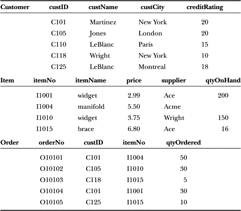
Source: ScienceDirect, customer table
Personality data
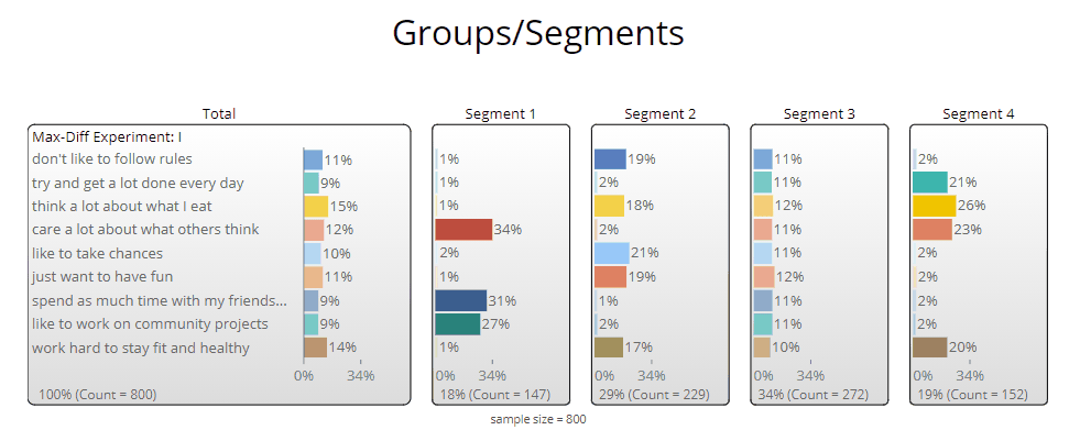
Source: Displayr help centre
Anomaly DetectionRows: patients. Columns: clinical features. The small group far from the rest is the one to look at
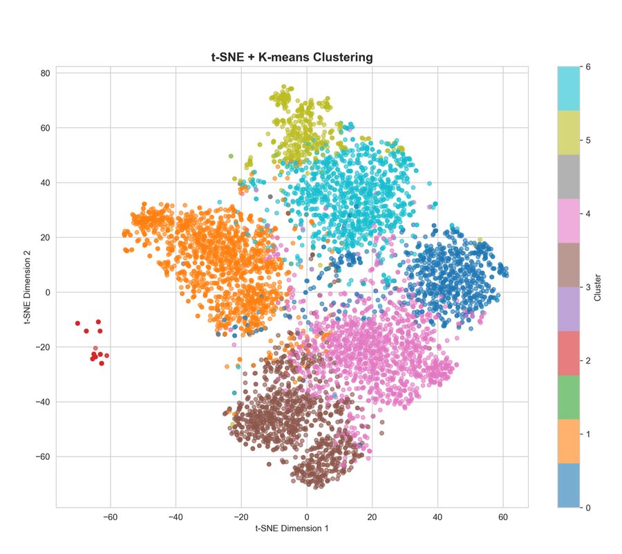
Source: Patient features from clinical reports, t-SNE and k-means (as on the original slide; publication not given)
Genetic AncestryRows: people. Columns: hundreds of thousands of genetic markers
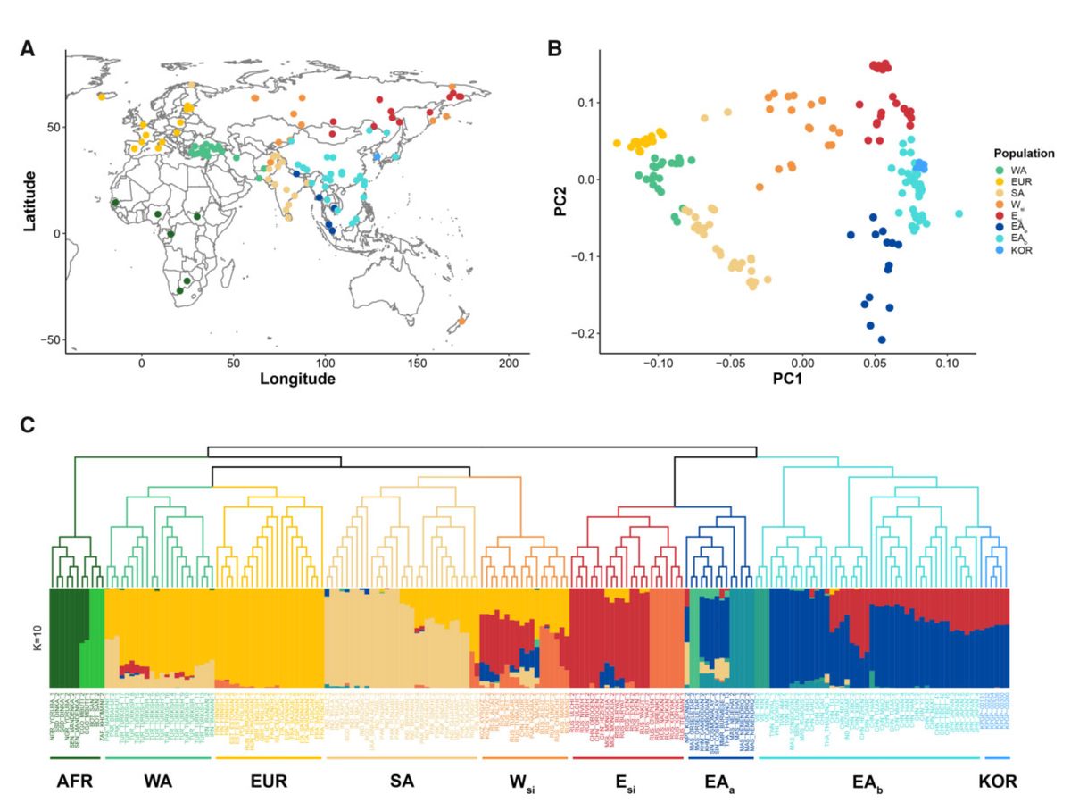
Palmer penguinsRows: 342 birds. Columns: four measurements. The species is in the file, and we hide it
| bill length | bill depth | flipper | mass | species |
|---|---|---|---|---|
| 39.1 | 18.7 | 181 | 3750 | hidden |
| 39.5 | 17.4 | 186 | 3800 | hidden |
| 40.3 | 18.0 | 195 | 3250 | hidden |
| … | … | … | … | … |
Millimetres and grams. The CSV has 344 rows; 2 have no measurements and are left out.
There are 151 Adelie, 68 Chinstrap and 123 Gentoo penguins. We pretend not to know this until k-means has answered.
One bird comes back in every part, the specimen: line 168 of the file, bill 45.9 mm by 17.1 mm, flipper 190 mm, 3575 g.
Data: Gorman, Williams and Fraser (2014), Palmer Station LTER, via palmerpenguins (CC0). Download the CSV.
Clustering · Gaussian Mixture ModelsOne way to describe groups: each is a Gaussian blob with its own centre and shape
A Gaussian mixture says how likely each point is to come from each blob. It is the subject of the next lecture; k-means, today, is its simplest relative.
Clustering · A zoo of clustering methodsEleven methods (columns) on six toy datasets (rows). Each draws different groups
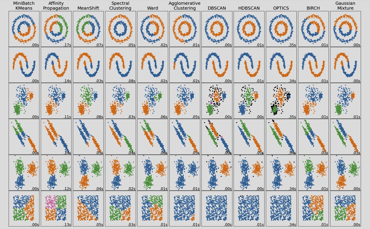
Source: scikit-learn, Clustering
Clustering · Hierarchical ClusteringMerge the two nearest groups, again and again: the dendrogram records the order
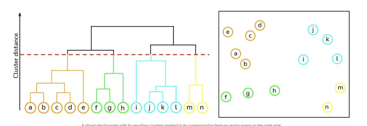
The height of each join is the distance between the two groups it merges. Cutting the tree at the red line gives the coloured groups.
Clustering · Hierarchical ClusteringCut the tree higher and there are fewer groups
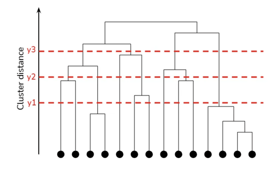
A cut at \(y_1\), \(y_2\) or \(y_3\) gives a different number of clusters from one tree, so the method does not need the number of clusters in advance.
Clustering · Hierarchical ClusteringThe levels of a tree can mean something
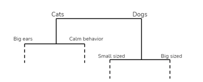
Cats and dogs at the top; big ears, calm behaviour, small or big size below. K-means gives one level only, and you choose which.
Part 2 of 5
K-means by hand
How does k-means find the groups?
K-Means ClusteringThe same 17 points. We want k = 2 groups
K-means describes each group by one point, its centre \(\mu_j\), and puts every \(x^{(i)}\) in the group of the nearest centre. The number of groups \(k\) is chosen by us.
K-Means Clustering · AlgorithmTwo steps, repeated
Initialize cluster centroids: \(\mu_1, \mu_2, \ldots, \mu_k \in \mathbb{R}^d\)
Repeat until convergence:
Assign. Each point goes to its nearest centre: \(c^{(i)} \in \{1, \ldots, k\}\) is the cluster of point \(i\).
Update. Each centre moves to the mean of its points. \(1\{c^{(i)} = j\}\) is 1 when point \(i\) is in cluster \(j\) and 0 otherwise, so the fraction is a sum over cluster \(j\) divided by its size.
K-Means ClusteringOne stage per click. Before the first assignment you can drag a centre and start somewhere else
K-Means Clustering · AlgorithmWhat you just watched, and the notation for this lecture and the next
Initialize cluster centroids: \(\mu_1, \mu_2, \ldots, \mu_k \in \mathbb{R}^d\)
Repeat until convergence:
| \(x^{(i)} \in \mathbb{R}^d\) | point \(i\), for \(i = 1, \ldots, n\) |
| \(k\) | the number of clusters, chosen by us |
| \(\mu_j \in \mathbb{R}^d\) | the centre of cluster \(j\), for \(j = 1, \ldots, k\) |
| \(c^{(i)}\) | the cluster of point \(i\), a number from 1 to \(k\) |
| \(J(c, \mu)\) | the distortion, next slide |
K-Means Clustering · Loss FunctionLoss that is being minimized
- K-means is coordinate descent on \(J(c, \mu)\), the distortion function: the assignment step minimizes \(J\) over \(c\) with \(\mu\) fixed, the update step over \(\mu\) with \(c\) fixed.
- \(J(c, \mu)\) is generally non-convex and susceptible to local minima.
- Problem can be fixed by trying different random initial values for \(\mu_j\).
| after assignment | \(J\) |
|---|---|
| 1 | 97.42 |
| 2 | 53.89 |
| 3 | 24.45 |
| 4 | 23.60 |
The walk-through's 17 points: \(J\) falls at every step and stops when no point changes cluster.
Why each step lowers JSo k-means always stops, though not always at the lowest J
- Assign. With the centres fixed, \(J\) is a sum of one term per point, and choosing the nearest centre makes each term as small as it can be. \( \lVert x^{(i)} - \mu_{c^{(i)}} \rVert^2 = \min_j \lVert x^{(i)} - \mu_j \rVert^2 \)
- Update. With the clusters fixed, the part of \(J\) for cluster \(j\) is a quadratic in \(\mu_j\). Its gradient is zero at the mean of the cluster. \( \nabla_{\mu_j} \sum_{i:\,c^{(i)} = j} \lVert x^{(i)} - \mu_j \rVert^2 = -2 \sum_{i:\,c^{(i)} = j} (x^{(i)} - \mu_j) = 0 \)
- So it stops. \(J\) never rises, and there are finitely many ways to assign \(n\) points to \(k\) clusters, so the assignments stop changing after a finite number of rounds.
See the CS229 notes, chapter 10 (cs229.stanford.edu), for the same argument.
K-means by handSix points on a line, two centres
The points are \(1, 2, 3, 7, 8, 12\). Start with \(\mu_1 = 2\) and \(\mu_2 = 3\).
- Assign each point to its nearest centre (a tie goes to \(\mu_1\)).
- Move each centre to the mean of its points.
- Repeat until nothing changes. How many updates did it take, and what is \(J\) at the end?
Do it on paper with your neighbour before the next slide.
K-means by hand · answer2 updates, then the assignment repeats
| round | \(\mu_1, \mu_2\) | \(c\) for 1, 2, 3, 7, 8, 12 | \(J\) |
|---|---|---|---|
| 1 | 2, 3 | 1 1 2 2 2 2 | 123 |
| 2 | 1.5, 7.5 | 1 1 1 2 2 2 | 23.5 |
| 3 | 2, 9 | 1 1 1 2 2 2 | 16 |
The first start is poor: both centres sit in the left group, so \(\mu_2\) must travel. After two updates the clusters are \(\{1, 2, 3\}\) and \(\{7, 8, 12\}\), with centres 2 and 9, and \(J = 16\).
Notice that 12 pulls the second centre to the right: a mean follows its farthest points.
Clustering · K-MeansEach centre (white cross) owns the region nearer to it than to any other centre
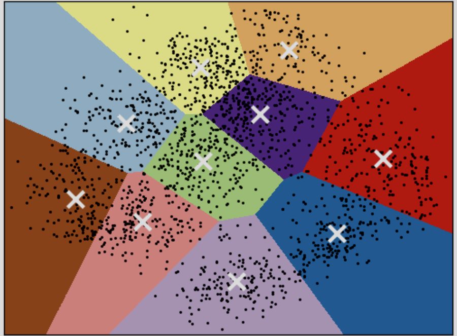
Source: scikit-learn, A demo of K-Means clustering on the handwritten digits data
The regions are convex polygons (a Voronoi diagram), and the border between two regions is the straight line halfway between their centres.
This is also how a new point is clustered: compare its distance to the centres, as on the last stage of the walk-through.
K-means in numpyThe code from the original slides: the data, the starting centres, the stopping rule
import numpy as np
import matplotlib.pyplot as plt
np.random.seed(0)

# define the dataset
n = 50
c1 = np.array([-3, -3])
c2 = np.array([2, 2])
sig = 1.2
data = np.concatenate([c1 + sig*np.random.randn(n, 2), c2 + sig*np.random.randn(n, 2)])

# initialize the centroids (as floats: an integer array would round every mean)
centroids = np.array([[-2, 3], [2, -3]], dtype=float)

max_iterations = 100           # define the maximum number of iterations
convergence_threshold = 1e-4   # define the convergence threshold
iteration = 0                  # initialize the iteration counter

# previous centroids: a random value different from the current centroids
prev_centroids = np.random.rand(2, 2)
Two clouds of 50 points around \((-3, -3)\) and \((2, 2)\). Run this block, then the loop on the next slide.
K-means in numpy · the loopAssign, update, until the centres stop moving. It prints J after each round
while np.sum(np.abs(prev_centroids - centroids)) > convergence_threshold and iteration < max_iterations:
    prev_centroids = centroids.copy()          # store the previous centroids
    clusters = np.zeros(len(data), dtype=int)  # initialize the cluster assignments

    # assign each data point to the closest centroid
    for i, point in enumerate(data):
        distances = np.sum((point - centroids)**2, axis=1)
        clusters[i] = np.argmin(distances)

    # update the centroids using the mean of the points in each cluster
    for j in range(2):
        centroids[j] = np.mean(data[clusters == j], axis=0)

    iteration += 1
    J = np.sum((data - centroids[clusters])**2)
    print(f'iteration {iteration}: J = {J:.2f}')

fig, ax = plt.subplots()
ax.scatter(data[:, 0], data[:, 1], c=['C0' if c == 0 else 'C1' for c in clusters], s=12)
ax.plot(centroids[:, 0], centroids[:, 1], 'x', color='C2', markersize=10)
ax.set_title('Last result')
plt.show()
It prints iteration 1: J = 1177.29; iteration 2: J = 298.71; iteration 3: J = 298.71.
Part 3 of 5
The penguins
What does k-means find in 342 penguins?
K-means on bill length and depthk = 3. Step it or run it, then show the species. Both axes in the same units
In millimetres the cloud is wide and flat, and k-means cuts it into vertical strips: 258 of 342 birds (75%) end up in their species' cluster.
Standardize firstA distance adds up the columns, so the column with the biggest numbers decides
Here \(m_t\) is the mean and \(s_t\) the standard deviation of column \(t\). Bill length spreads over 5.5 mm (one standard deviation) and bill depth over 2.0 mm, so in millimetres a difference in length counts almost three times as much. After standardizing, every column has mean 0 and spread 1.
With four columns it is worse: body mass is in grams (spread 801 g) and carries 99.96% of the total spread, so k-means on raw numbers clusters by weight alone.
| k = 3 on | raw | standardized |
|---|---|---|
| bill length and depth | 75% | 93% |
| all four measurements | 58% | 92% |
| one measurement alone (best: flipper length) | 76% | |
Share of the 342 birds in the cluster matched to their species, best of 50 starts.
Four measurementsClustered in four dimensions; look through any two of them
Gentoo is found perfectly. But 24 Adelie join the Chinstraps, and the total, 92%, is no better than two measurements gave (93%). More columns are not more information about the species when the new ones separate something else.
Which centre is nearest?The three regions on standardized bills. Click any bird
The penguins in numpyStandardize, 20 random starts, keep the lowest J, then compare with the species
import numpy as np
import pandas as pd

d = pd.read_csv('penguins.csv').dropna(subset=['bill_length_mm', 'bill_depth_mm'])
X = d[['bill_length_mm', 'bill_depth_mm']].values
Z = (X - X.mean(axis=0)) / X.std(axis=0)          # standardize: mean 0, spread 1

def kmeans(Z, k, rng):
    mu = Z[rng.choice(len(Z), k, replace=False)]   # k random birds as the first centres
    while True:
        D = ((Z[:, None, :] - mu[None, :, :])**2).sum(axis=2)   # n by k squared distances
        c = D.argmin(axis=1)                                     # assignment step
        new = np.array([Z[c == j].mean(axis=0) for j in range(k)])  # update step
        if np.allclose(new, mu):
            return c, mu, D[np.arange(len(Z)), c].sum()          # J, the distortion
        mu = new

rng = np.random.default_rng(0)
runs = [kmeans(Z, 3, rng) for _ in range(20)]    # 20 restarts, keep the lowest J
c, mu, J = min(runs, key=lambda r: r[2])
print(f'J = {J:.1f}')
print(pd.crosstab(c, d.species))                 # the species were never used above
It prints J = 186.9 and the table of clusters against species (317 of 342 on the diagonal of the best matching).
Part 4 of 5
How many clusters?
How many groups are really there?
The elbowJ always falls as k grows. Look for where it stops falling fast. Click a k
On bills, J drops by 344, then 153, then only 39: an elbow at 3. On all four the drops are 802, 186, 79: the bend at 2 is sharper than at 3.
The silhouetteFor each point: is it nearer its own cluster than the next one?
\(a(i)\) is the mean distance from point \(i\) to the other points of its cluster, \(b(i)\) the mean distance to the points of the nearest other cluster. \(s\) near 1: well inside; near 0: on a border; negative: probably in the wrong cluster.
The mean silhouette is highest at k = 3 on bills (0.52) but at k = 2 on all four (0.53). The specimen sits on a border: \(s = 0.00\).
Two, three or six?The four measurements, clustered with k = 2, 3 and 6, against species and sex
Every one of these answers is a real structure in the birds. Gentoo against the rest is the strongest split; the species are next; then males and females, who differ in size.
The data cannot say which grouping you meant. The elbow and the silhouette measure how separated the groups are, and that is a different question from what a kind is.
The class, clusteredYour four answers, standardized, k-means with the k you pick. What does each cluster mean?
In teams: argue for one k, and give each cluster a name from its centre. Then ask whether the groups are in the room or only in the method.
Part 5 of 5
Where it breaks
When does k-means split the data wrong?
Where you start mattersk = 3 on the four standardized measurements, from 1,000 different starts
From three random birds, 152 of 1,000 runs stop at \(J \approx 486\), a local minimum, instead of \(J = 379.4\). Each run did everything right: every step lowered \(J\).
The fix on the original slide: try several starts and keep the lowest \(J\).
k-means++Spread the starting centres out: each new one is drawn far from the others
| 1,000 starts, four measurements | random | k-means++ |
|---|---|---|
| mean J of the start | 1129 | 842 |
| mean number of updates | 6.4 | 5.5 |
| runs stuck near J = 486 | 152 | 180 |
Honest result: on the penguins k-means++ starts lower and finishes sooner, but it lands in the bad minimum as often as random starts. Its guarantee (Arthur and Vassilvitskii, 2007) is about the average J, within a factor of order \(\log k\) of the best; restarts are still needed.
Tilted clustersEach species is a tilted ellipse. K-means can only cut with straight lines halfway between centres
Over all birds, longer bills are shallower (correlation −0.24). Inside each species it is the other way round: +0.39, +0.65, +0.64 for Adelie, Chinstrap and Gentoo. That is Simpson's paradox, and it is what tilts the three clouds.
K-means measures distance the same way in every direction, so it assumes round clusters of the same size. The 25 ringed birds are those the straight borders cut off from their species; the specimen is one of them, almost exactly on a border.
A small groupKeep fewer Chinstraps and cluster again with k = 3
With all 68, the Chinstrap cluster holds 54 of them. With 17, it still holds all 17, but it has grown to 49 birds, mostly Gentoo. With 10, k-means splits the Adelie in two instead and the Chinstraps have no cluster at all.
J counts every bird once, so splitting a big group lowers it more than finding a small one. K-means prefers clusters of similar size and spread.
Next: why does k-means split the penguins wrong?A cluster with its own shape
Replace each round centre by a Gaussian with its own covariance, a tilted ellipse of any size, and assign each bird by probability instead of distance. On the same standardized bills, a Gaussian mixture puts 330 of 342 birds (96%) with their species, against 317 for k-means, and the specimen goes back to the Chinstraps.
How a mixture is fitted (the EM algorithm, k-means with soft assignments) is the next lecture. The notation stays: \(x^{(i)}\), \(\mu_j\), \(k\); the assignment \(c^{(i)}\) becomes a probability.
Takeaways
- K-means alternates two steps, assign each point to its nearest centre and move each centre to its mean, and each step lowers the distortion J.
- Distances add up the columns, so standardize first: on the penguins that alone moves the match with the species from 75% to 93%.
- The elbow and the silhouette measure separation, not meaning: the penguins have a good answer at 2, 3 and 6.
- K-means finds round clusters of similar size, from wherever it starts: restart it, and expect it to miss tilted or small groups.